Changing the Center of Gravity: Transforming Classical Studies Through Cyberinfrastructure
2009
Volume 3 Number 1
Abstract
We describe two different strategies for generating the morphology of Latin verbs. First, we hand-code default inheritance hierarchies in the KATR formalism, treating inflectional exponents as markings associated with the application of rules by which complex word
forms are deduced from simpler roots or stems. The high degree of similarity among verbs of different conjugation classes allows us to formulate general rules; these general rules are, however, sometimes overridden by conjugation-specific rules. This approach allows linguists to gain an appreciation for the structure of verbs, gives teachers a foundation for organizing lessons in morphology, and provides students a technique for generating forms of any verb. Second, we start with a paradigm chart, then automatically remove common parts and redundant morphosyntactic property sets (columns), combine similar conjugations (rows), and generate the KATR theory that produces a complete table of forms for a set of lexemes. This second approach automatically determines principal parts (for Latin, we verify that there are four), groups inflection classes into super-classes, and builds full paradigm charts.
Introduction
Recent research into the nature of morphology has demonstrated the feasibility of two alternative approaches to the definition of a language’s inflectional system. Central to both approaches is the notion of an inflectional paradigm. In general terms, the
inflectional paradigm of a lexeme L can be regarded as a set of
cells
[1], where each cell is the pairing of L with a set
of morphosyntactic properties, and each cell has a word form as its realization; for instance, the paradigm of the lexeme
walk includes cells such as
<WALK, {3rd singular present indicative}> and
<WALK, {past}>,
whose
realizations are the word forms
walks and
walked.
Given this notion, one approach to the definition of a language’s inflectional system is the
realizational approach (see [
Matthews 1972], [
Zwicky 1985], [
Anderson 1992], [
Corbett 1993], [
Stump 2001]). In this approach, each
word form in a lexeme’s paradigm is deduced from the lexical and morphosyntactic properties of the cell that it realizes by means of a system of
morphological rules. For instance, the word form
walks is deduced from
the cell <WALK, {3rd singular present indicative}> by means of the rule of
-s suffixation, which applies to the root
walk of the lexeme WALK to express
the property set {3rd singular present indicative}.
An alternative approach to the definition of a language’s inflectional
system is the
implicative approach (see [
Blevins 2005], [
Blevins 2006], [
Finkel 2009]). According to this approach, certain word forms in a lexeme’s
paradigm serve as the basis for inferring the paradigm’s other forms. In
Old English, for instance, the word form
hældon
“healed (plural)” may be
deduced from the word form
hælde
“healed (3rd singular)” in accordance
with a general principle that in the inflection of a weak verbal lexeme L, the
realization of <L, {3rd singular past indicative}> and that of <L, {plural
past indicative}> stand in the relation
Xde ↔
Xdon.
Despite their differences, both approaches are capable of generating
a language’s inflected forms. We demonstrate this claim for Latin. We
first present a realizational analysis of Latin in the KATR language [
Finkel 2002]. KATR is based on DATR, a formal language
for representing lexical knowledge designed and implemented by Roger
Evans and Gerald Gazdar [
Evans 1989]. We then present an implicative analysis that uses techniques of abstraction and grouping to derive both a principal-part analysis and a different KATR theory for Latin.
This research is part of a larger effort aimed at elucidating the morphological structure of natural languages. In particular, we are interested in
identifying the ways in which default-inheritance relations describe a language’s morphology as well as the theoretical relevance of the traditional
notion of principal parts.
Benefits
As we demonstrate below, the realizational approach leads to a Latin KATR
theory that provides a clear picture of the morphology of Latin verbs. Different audiences might find different aspects of it attractive.
- A linguist can peruse the theory to gain an appreciation for the structure of Indo-European verbs in general and Latin verbs in particular,
with all exceptional cases clearly marked either by morphophonological
diacritics or by rules of sandhi, which are segregated from all the other rules.
- A teacher of the language can use the theory as a foundation for organizing lessons in morphology.
- A student of the language can suggest verb roots and use the theory
to generate all the appropriate forms, instead of locating the right
paradigm in a book and substituting consonants.
The implicative approach that we demonstrate in this paper has several
benefits.
- It automatically determines which forms of a verb could be treated
as principal parts. For Latin, we compute that four principal parts
suffice.
- It allows us to group inflection classes into super-classes. For Latin
verbs, there are more than four inflection classes if one takes into
account variations in such forms as those of the active perfect and
passive participle; our grouping method shows that the traditional
organization into four conjugations is consistent with super-classes
of our more finely detailed set of inflection classes.
- It generates charts showing the full paradigm of lexemic exemplars;
such charts can have pedagogic value.
A Realizational KATR Theory for Latin
The purpose of the KATR theory described here is to generate verb forms
for Latin, specifically, the realizations of all combinations of the morphosyntactic properties of voice (active/passive), mood (indicative/subjunctive),
aspect (imperfective/perfective), tense (present/past/future), number (singular/plural), and person (1/2/3). The combinations form a total of 144
morphosyntactic property sets (MPSs). However, Latin has no future subjunctive, reducing the total to 120 MPSs.
Latin verbs consist of a sequence of morphological formatives, arranged
in five slots:
- Root, which realizes the verb’s lexeme, possibly dependent on the
aspect. For instance, for the verb laudō, the stem is laud.
- Tense marker 1, which realizes part of the verb’s tense, possibly dependent on the mood. For instance, for past perfective subjunctive,
this marker is issē.
- Tense marker 2, which realizes another part of the verb’s tense. This
marker is usually empty. For the past indicative, though, it is ā, and
for the present perfective subjunctive, it is ī.
- Person/Number, which realizes a verb’s properties of person and
number, possibly dependent on other categories. For example, the
marker for the first person singular present indicative is ō.
- Voice, which realizes a verb’s voice. It is empty for the active voice,
and is usually r for the passive voice.
To keep our discussion short, we omit the imperative and infinitive forms,
although our complete KATR theory includes them without difficulty. For
those forms that use a participle (such as the perfective passive), we limit
ourselves to a single form, the masculine singular.
There are four frequently encountered conjugations, distinguished by
their theme vowel: first (ā: laudāre), second (ē: monēre), third (i: dūcere,
capere), fourth (ī: audīre). The third conjugation has two variants; in one (capere), the theme vowel is more pronounced.
The Conjugation-1 Verb laudāre “Praise”
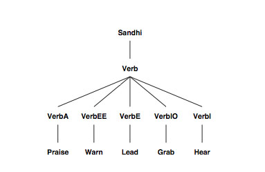
A theory in KATR is a network of
nodes. The network of nodes constituting our verb morphology theory is partially represented in Figure 1. The organizational principle in this network is hierarchical: The tree structure’s
terminal nodes represent individual verbal lexemes, and each of the non-terminal nodes in the tree defines default properties shared by the lexemes
that it dominates.
Each of the nodes in a theory houses a set of
rules. We represent the
verb
laudāre
“praise” by a node:
Praise:
  1 <root> == l a u d
  2 <> == VerbA
The node, named
Praise, has two rules, which we number for discussion purposes only. KATR syntax requires that a node be terminated
by a single period (full stop), which we omit here. Our convention is to
name the node for a lexeme by a capitalized English word (here
Praise)
representing its meaning.
Rule 1 says that a query asking for the root of this verb should produce a
four-atom result containing l, a, u, and d. Rule 2 says that all other queries
are to be referred to the VerbA node, which we introduce below.
A query is a list of atoms, such as <root> or <active indicative perfect present 1 sg>, addressed to a node such as Praise. In our
theory, the atoms in queries generally represent morphological formatives
(such as root, themeVowel), morphosyntactic properties (such as perfect, sg) or surface forms (specific orthographic characters).
A query addressed to a given node is matched against all the rules
housed at that node. A rule matches if all the atoms on its left-hand side
match the atoms in the query. A rule can match even if its atoms do not exhaust the entire query. In the case of Praise, a query <root perfect>
is matched by Rules 1 and 2; a query <themeVowel> is only matched by
Rule 2.
Left-hand sides expressed with path notation (<pointed brackets>)
only match if their atoms match an initial substring of the query. Left-hand
sides expressed with set notation ({braces}) match if their atoms are all
expressed, in whatever position, in the query. We usually use set notation
for queries based on morphological formatives and morphosyntactic properties, where order is insignificant, but path notation for queries based on
surface forms, where order is significant.
When several rules match, KATR picks the best match, that is, the one
whose left-hand side “uses up” the most of the query. This choice embodies Pāṇini’s principle, which entails that if two rules are applicable, the
more restrictive rule applies, to the exclusion of the more general rule. We
sometimes speak of a rule’s Pāṇini precedence, which is the cardinality of
its left-hand side. If a node in a KATR theory houses two applicable rules
with the same Pāṇini precedence, we consider that theory malformed.
In our case, Rule 2 of
Praise only applies when Rule 1 does not apply,
because Rule 1 is always a better match if it applies at all. Rule 2 is called a
default rule, because it applies by default if no other rule applies. Default
rules define a hierarchical relation among some of the nodes in a KATR
theory; thus, in the tree structure depicted in
Figure 1, node X immediately
dominates node Y iff Y houses a default rule that refers queries to X.
KATR generates output based on queries directed to nodes representing individual lexemes. Since these nodes, such as Praise, are not referred to by other nodes, they are called leaves, as opposed to nodes like VerbA,
which are called internal nodes. The KATR theory itself indicates the list
of queries to be addressed to all leaves. Here is the output that KATR generates for several queries directed to the Praise node.
|
active,indicative,imperfective,present,sg,1
|
laudō
|
|
active,indicative,imperfective,past,sg,2
|
laudābās
|
|
active,indicative,imperfective,past,sg,3
|
laudābat
|
|
active,indicative,imperfective,future,pl,1
|
laudābimus
|
|
active,indicative,perfective,present,pl,2
|
laudāvistis
|
|
active,indicative,perfective,past,pl,3
|
laudāverant
|
|
active,indicative,perfective,future,sg,1
|
laudāverō
|
|
active,subjunctive,imperfective,present,sg,2
|
laudēs
|
|
active,subjunctive,imperfective,past,sg,3
|
laudāret
|
|
active,subjunctive,imperfective,past,pl,1
|
laudārēmus
|
|
active,subjunctive,perfective,present,pl,2
|
laudāverītis
|
|
passive,indicative,imperfective,present,pl,3
|
laudantur
|
|
passive,indicative,imperfective,past,sg,1
|
laudābāmer
|
|
passive,indicative,imperfective,past,sg,2
|
laudābāris
|
|
passive,indicative,imperfective,future,sg,3
|
laudābitur
|
|
passive,indicative,perfective,present,pl,1
|
laudātīsumus
|
|
passive,indicative,perfective,past,pl,2
|
laudātīerātis
|
|
passive,indicative,perfective,future,pl,3
|
laudātīerunt
|
The rule for
Praise illustrates the strategy we term
provisioning
[
Finkel 2007b]: It provides information (here, the consonants of the verb’s
root) needed by but not provided by more general nodes (here,
VerbA and
the nodes to which it, in turn, refers).
We refer to the individual segments of a morphological form by means
of particular atoms:
-
themeVowel is the vowel usually found after the root of a verb.
- The atoms stemImperfective, stemPerfective, and stemParticiple are the verb stems, usually including the theme vowel, that precede suffixes marking tense, number, person, mood, and aspect.
The VerbA Node
We now turn to the
VerbA node, to which the Praise node refers.
VerbA:
         1 <themeVowel> == ā
         2 <stemImperfective> == "<oot>" <themeVowel>
         3 <stemPerfective> == <stemImperfective> v
         4 <stemParticiple> == <stemImperfective> t
         5 <> == Verb:<conj1>
As with the
Praise node,
VerbA defers most queries to its parent, in this case the node called
Verb, as Rule 5 indicates.
Most of these rules are for provisioning. Rule 1 answers the
themeVowel query. We sometimes address this query to leaf nodes; the Praise node defers it to VerbA, which answers the query.
Rules 2-4 provision the three stems. The quoted path <root> in the
right-hand side directs a new query to the node to which the original query
was first addressed, in our case, Praise, which produces the four atoms
l a u d. The non-quoted path <themeVowel> directs a new query to the
current node, that is, VerbA, resolved by Rule 1. The right-hand side of the
rule in this case is equivalent to l a u d ā. Similarly, the right-hand side of Rule 3 is l a u d ā v, and the right-hand side of Rule 4 is l a u d ā t.
Rule 5 is a default rule, directing its query to the Verb node, with the
atom conj1 prepended to the query. Therefore, queries addressed to Verb contain not only morphosyntactic markers (such as “present passive”) but
also informational markers (“conj1”).
By way of contrast, we also present the
VerbIO node, which applies to
i-stem third-conjugation verbs such as
facere and
capere.
VerbIO:
       1 {themeVowel} == i
       2 {themeVowel past imperfective } == I
       3 {themeVowel 2 sg present imperfective passive
       indicative} == I
       4 {themeVowel imperative} == I
       5 {themeVowel infinitive} == I
       6 <stemImperfective> == "<root>" <themeVowel>
       7 <stemPerfective> == AEE:<"<root>">
       8 <stemParticiple> == "<root>" t
       9 <> == Verb:<conj3io>
Rules 2-5 introduce the strategy we call
overriding, answering a query
that is usually answered by a more general node in order to provide specific results for this situation. The left-hand sides of these rules use braces
instead of angle brackets, indicating that the order of appearance of the
atoms is irrelevant for matching the rules. The atom I that appears on
the right-hand sides of these rules is a
morphophoneme that either disappears or converts to an
i or an
e, depending on surrounding context, during a postprocessing step.
Rule 7 introduces the
lookup strategy, by which particular information
is obtained by reference to a special-purpose node. It directs a query such
as
f a c to the
AEE node to convert the
a to
ē, so the perfective stem of
facere becomes
fēc. Here is that lookup node:
AEE:
  1 <$letter#1 a $letter#2> == $letter#1 ē $letter#2
This node depends on a definition (not shown) that defines what atoms
are in the category “letter.” Rule 1 says that any query beginning with a
letter, then the atom
a, then any letter, should evaluate to the two letters
surrounding
ē instead.
The Verb Node
Queries addressed to
Praise are generally deferred to its parent,
VerbA, which then defers them further to
Verb.
Verb:
       1 {$conj34 1 sg future/present imperfective
           indicative/subjunctive} =+= <>
       2 {future subjunctive} == !
       3 {perfective passive} == Sandhi:<"<stemParticiple>"
           AdjSuffix:<nominative masculine> wordEnd> ,
           ToBe:<imperfective active>
       4 <> == Sandhi:<StemAspect SuffixTense1 SuffixTense2
           SuffixPersonVoice wordEnd>
Rule 1 reflects the future indicative to the present subjunctive in verbs
of conjugations 3 and 4 (abbreviated by the value
$conj34) in the first singular imperfective. This rule is quite specialized, applying, for instance,
to
dūcam
“I will lead / may I lead.” Without this rule, we would produce
dūcēo
“I will lead.”
Rule 2 indicates that there is no result for a query involving future subjunctive forms; Latin does not have these forms.
Rules 3 and 4 reflect to the Sandhi node as a postprocessing step after
assembling the components of a verb. The rule with the widest applicability, Rule 4, is the default rule. It combines the results of queries directed to the four nodes StemAspect, SuffixTense1, SuffixTense2, and SuffixPersonVoice, along with the marker wordEnd for postprocessing. Rule 3 generates forms for the perfective passive, which involve a participle, an adjectival end, and a specific form of the verb esse, which has its own node ToBe.
Auxiliary Nodes
The
Verb node invokes several auxiliary nodes.
StemAspect:
         1 {imperfective} =+= "<stemImperfective>"
         2 {perfective} =+= "<stemPerfective>"
The stem depends on the aspect; it either results in the imperfective
or the perfective stem. The
=+= notation preserves all the elements of the
query path, including those otherwise removed by matching the left-hand
side of the rules.
SuffixTense1:
         1 <> ==
         2 {conj1 present imperfective subjunctive} == ē
         3 {present imperfective subjunctive} == ā
         4 {perfective} == e r
         5 {past perfective subjunctive} == i s s ē
         6 {present perfective indicative} == I
         7 {3 pl present perfective indicative} == ē r
         8 {3 pl present perfective subjunctive} == e r
         9 {past imperfective indicative} == b
         10 {future imperfective indicative} == b
         11 {past imperfective indicative conj3io} == i ē b
         12 {past imperfective indicative conj4} == ē b
         13 {future imperfective indicative $conj34} ==
         14 {future imperfective indicative conj4} == ē
         15 {future imperfective indicative conj3io} == ē
         16 {past imperfective subjunctive} == r ē
The
SuffixTense1 node contains most tense information. It ranges
from very specific rules, like Rule 14, to fairly general rules, such as Rule 4,
which is overridden by more specific Rules 5-8.
SuffixTense2:
         1 {past indicative} == ā
         2 {present perfective subjunctive} == ī
         3 <> ==
The second tense suffix is usually empty (Rule 3), but it is occasionally
either
ā or
ī.
SuffixPersonVoice:
         1 {2 sg} == I SuffixVoice SuffixPerson
         2 {2 pl passive} == I m i n ī
         3 <> == SuffixPerson SuffixVoice
The suffix for person and voice is occasionally quite specific, as in the
second person plural passive. In the second person singular, the voice suffix (
r for the passive) precedes the person suffix, as in
laudāris
“you (sg) are
praised,” whereas the voice suffix usually follows the person suffix, as in
laudāmur
“we are praised.”
SuffixVoice:
         1 {passive} == r
         2 {passive 3} == u r
         3 <> ==
In general, Rule 3 indicates that there is no suffix for voice. However,
there is a suffix for the passive voice, which is generally
r (Rule 2) but sometimes
ur (Rule 3).
SuffixPerson:
         1 {1 sg} == m
         2 {1 sg present imperfective indicative} == ō
         3 {1 sg future indicative} == ō
         4 {1 sg present perfective indicative} == ī
         5 <> == SuffixalVowel Desinence
The personal suffix is usually a vowel and a
desinence (Rule 5), but
the first person singular is exceptional, with a general suffix
m (Rule 1) but
sometimes
ō or
ī.
SuffixalVowel:
         1 {future} == I
         2 {present imperfective indicative} == I
         3 {past imperfective subjunctive} == I
         4 {3 pl +2} == u
         5 {3 pl future perfective active} == I
         6 <> ==
The vowel has several forms; sometimes it is the morphophoneme
I
as in
laudābit
“he will praise,” but sometimes
u, as in
laudābunt
“they will
praise.”
Desinence:
         1 {2 sg} == I s
         2 {2 sg present perfective indicative} == s t ¯ı
         3 {3 sg} == t
         4 {1 pl} == m u s
         5 {2 pl} == t i s
         6 {2 pl present perfective indicative} == s <2 pl>
         7 {3 pl} == n t
The desinence provides the final consonants, typically marking person
and number, but occasionally influenced by aspect and tense (Rules 2 and
6).
The Sandhi Node
After we assemble the entire verb, we apply language-specific sandhi rules
to account for phonological alterations.
Sandhi:
         1 <wordEnd> ==
         2 <$letter> == $letter <>
         3 <s r wordEnd> == <r wordEnd>
         4 <I> == <i>
         5 <$unroundedVowel I> == <$unroundedVowel>
         6 <I r> == >e r>
         7 <I $longUnroundedVowel> == $longUnroundedVowel>
         8 <I e wordEnd> == e % canIe => cane
         9 <i i> == <i> % cap i i ē bam -> capieebam
         10 <ā ō> == ¯o>
         11 <ā ē> == <ē>
         12 <ē ō> == <e ō>
         13 <ē ā> == <e ā> % moneeām -> moneām
         14 <ī ō> == <i ō> % audīoo -> audioo
         15 <ī ē> == <i ē> % audīees -> audiees
         16 <ī ā> == <i ā> % audīām -> audiām ->
         17 <ī ū> == <i ū> % audīūnt -> audiūnt
         18 <ū $vowel> == <u $vowel> % frūctū-um ->
             frūctu-um; cornūa->
         19 <$longVowel $nonSibilantConsonant wordEnd> ==
             <Shorten:<$longVowel> $nonSibilantConsonant wordEnd>
         20 <$longVowel $stop#1 $stop#2> ==
             <Shorten:<$longVowel> $stop#1 $stop#2>
         21 <$longUnroundedVowel u> ==
             <$longUnroundedVowel> % dūceebāunt ->
             dūceebānt -> ..
         22 <c s> == <x>
         23 <g s> == <c s>
         24 <$consonant r wordEnd> == <$consonant e r
             wordEnd>
Unlike other nodes,
Sandhi works strictly from left to right, dealing
with a few atoms at a time. The first rule removes the
wordEnd marker
if that is all that is left. The other rules simplify the beginning of the remaining string of letters and then use angle brackets to direct the modified
string back to the
Sandhinode.
Rule 2 is quite general: if no more specific rule applies, it takes a single
letter from the query as output, and directs the remainder of the query
back to Sandhi. Rule 3 converts forms like *dūcimusr to *dūcimur. Rules 4-8 deal with the morphophoneme I, typically converting it to i (Rule 5),
but sometimes converting it to e or removing it entirely. Rules 9-18 deal
with two vowels in a row; typically, the second vowel is retained, and the
first either disappears or shortens. Rules 19 and 20 shorten long vowels
in certain contexts by applying to the Shorten rule, which we omit here.
Finally, Rules 22-24 introduce spelling rules. We include them in under the
rubric of sandhi.
Strategies for Building KATR Theories
We have been applying KATR to natural-language morphology for several years. In addition to Latin, we have built a complete morphology of
Hebrew verbs [
Finkel 2007b], large parts of Sanskrit (and other
related languages), and smaller studies of Bulgarian, Swahili, Georgian,
Lingala, Spanish, Polish, and Turkish. KATR allows us to represent morphological rules for these languages with great elegance.
Writing specifications in KATR is not easy. KATR is capable of representing elegant theories, but arriving at those theories requires considerable effort. Early choices color the structure of the resulting theory, and the author must often discard attempts and rethink how to represent the target morphology. The hardest choice is often whether to model a form by introducing a sandhi rule or a formative rule. An example is the
-mur suffix that
marks first person plural passive. We choose to model this ending as
mus
+ r and to reduce the result by sandhi. We could have introduced instead
a rule in the
Desinence node:
4.5 {1 pl passive} = m u
and let the
r appear due to the
SuffixVoice node. In this case, we prefer
not to introduce a special rule in
Desinence, partially because it looks so
similar to the existing Rule 4, and therefore seems unparsimonious, and
partially because we hypothesize that historically there really was some
form
*-musr that eventually elided the two final consonants.
An Implicative KATR Theory for Latin
The Paradigm Chart
We start this analysis by presenting a paradigm of word forms for Latin
verbs. Table 2 displays a subset of the entire paradigm that covers only
the present indicative active forms. The roots of lexemes are abstracted
away from this paradigm.
| CONJ |
PrIAc1s |
PrIAc2s |
PrIAc3s |
PrIAc1p |
PrIAc2p |
PrIAc3p |
| TEMPLATE |
4S1C |
1S1Cs |
1S1Ct |
4S1Cmus |
1S1Ctis |
4S1Cnt |
| cIa |
ō |
ā |
ā |
ā |
ā |
ā |
| cIb |
ō |
ā |
ā |
ā |
ā |
ā |
| cIc |
ō |
ā |
ā |
ā |
ā |
ā |
| cIIa |
eō |
ē |
ē |
ē |
ē |
ē |
| cIIb |
eō |
ē |
ē |
ē |
ē |
ē |
| cIIc |
eō |
ē |
ē |
ē |
ē |
ē |
| cIId |
eō |
ē |
ē |
ē |
ē |
ē |
| cIIe |
eō |
ē |
ē |
ē |
ē |
ē |
| cIIIa |
ō |
i |
i |
i |
i |
i |
| cIIIb |
ō |
i |
i |
i |
i |
i |
| cIIIc |
ō |
i |
i |
i |
i |
i |
| cIIId |
ō |
i |
i |
i |
i |
i |
| cIIIe |
iō |
i |
i |
i |
i |
i |
| cIIIf |
ō |
∅ |
∅ |
∅ |
∅ |
∅ |
| cIIIs |
um |
∅ |
∅ |
u |
∅ |
u |
| cIVa |
iō |
ī |
ī |
ī |
ī |
ī |
| cIVb |
iō |
ī |
ī |
ī |
ī |
ī |
| cIVc |
iō |
ī |
ī |
ī |
ī |
ī |
| cIVd |
iō |
ī |
ī |
ī |
ī |
ī |
Table 2.
Latin paradigm fragment (6 of the 92 columns)
We have expanded the traditional four conjugations into 19 conjugations. They are mostly distinguished by forms not shown here, particularly by the perfect indicative active. For instance, a cIa verb such as iuvāre
“help” forms the perfect stem by lengthening the middle vowel, as in iūvī
“I helped,” whereas a cIb verb such as laudāre
“praise” simply adds āvī to the stem to form the perfect 1 singular. For completeness, we even include conjugation cIIIs for the two exceptional verbs esse
“be” and posse
“be able.”
The line marked CONJ simply lists the morphosyntactic property sets
for our convenience.
The line marked TEMPLATE indicates parts of the chart that are constant
within each column. For instance, the second-person singular is marked
with 1S1Cs. The 1S part means “place the first stem here.” We choose to
make the first stem the present stem. Next, 1C means “place the first entry in the column here.” Our Latin charts have only a single entry per column
in each row. When an entry is empty, we mark it with ∅. Finally, s means
“place the letter s here”. All Latin verbs follow this strategy for building
the perfect indicative active 2nd person singular forms.
Our chart requires that each verb have five stems, possibly identical: present, perfect, supine, present first person, and present past subjunctive. For iuvāre “help,” these stems are iuv, iū, iū, iuv, and iuv, respectively. For esse “be,” the stems are es, fu, es, s, and es, respectively.
It often happens that a conjugation regularly refers one stem to another. For instance, class cIa refers the fourth and fifth stems to the first; class cIIIs refers the third to first. (For consistency, we always refer stems to earlier-numbered stems.) We represent stem referrals as an addendum to our chart, as in Table 3.
| REFER |
cIa 4 , 5 -> 1 |
| REFER |
cIb 2 - 5 -> 1 |
| REFER |
cIc 2 - 5 -> 1 |
| REFER |
cIIa 2 - 5 -> 1 |
| REFER |
cIIb 2 - 5 -> 1 |
| REFER |
cIIc 2 - 5 -> 1 |
| REFER |
cIId 4 , 5 -> 1 ; 3 -> 2 |
| REFER |
cIIe 4 , 5 -> 1 |
| REFER |
cIIIa 2 - 5 -> 1 |
| REFER |
cIIIb 2 - 5 -> 1 |
| REFER |
cIIIc 2 - 5 -> 1 |
| REFER |
cIIId 2 - 5 -> 1 |
| REFER |
cIIIs 3 -> 1 |
| REFER |
cIIIe 3 - 5 -> 1 |
| REFER |
cIVa 3 - 5 -> 1 |
| REFER |
cIIIf 4 - 5 -> 1 |
| REFER |
cIVb 2 - 5 -> 1 |
| REFER |
cIVc 2 - 5 -> 1 |
| REFER |
cIVd 2 - 5 -> 1 |
Table 3.
Latin stem referrals
We then represent the lexicon by indicating the conjugation and stems of each verb as another addendum to the chart, as in Table 4.
| LEXEME |
help |
cIa |
1:iuv |
2:ded |
3:iū |
| LEXEME |
bathe |
cIa |
1:lav |
2:lāv |
3:lau |
| LEXEME |
stand |
cIa |
1:st |
2:stet |
3:sta |
| LEXEME |
give |
cIa |
1:d |
2:ded |
3:da |
| LEXEME |
praise |
cIb |
1:laud |
| LEXEME |
rattle |
cIc |
1:crep |
| LEXEME |
destroy |
cIIa |
1:dēl |
| LEXEME |
mourn |
cIIb |
1:lūg |
| LEXEME |
order |
cIIb |
1:iub |
| LEXEME |
warn |
cIIc |
1:mon |
| LEXEME |
see |
cIId |
1:vid |
2:vīd |
| LEXEME |
arouse |
cIIe |
1:ci |
2:cī |
3:ci |
| LEXEME |
decide |
cIIIa |
1:dēcern |
| LEXEME |
nourish |
cIIIb |
1:al |
| LEXEME |
lead |
cIIIc |
1:dūc |
| LEXEME |
attach |
cIIId |
1:fīg |
| LEXEME |
take |
cIIIe |
1:cap |
2:cēp |
| LEXEME |
carry |
cIIIf |
1:fer |
2:tul |
3:lāt |
| LEXEME |
be |
cIIIs |
1:es |
2:fu |
4:s |
|
| LEXEME |
be able |
cIIIs |
1:potes |
2:possu |
4:poss |
5:pos |
| LEXEME |
go |
cIIIs |
1:i |
2:i |
4:e |
5:ī |
| LEXEME |
come |
cIVa |
1:ven |
2:vēn |
| LEXEME |
hear |
cIVb |
1:aud |
| LEXEME |
leap |
cIVc |
1:sal |
| LEXEME |
bind |
cIVd |
1:vinc |
The final section of the paradigm chart expresses rules of sandhi, as shown in Table 5.
| CLASS |
finalStop r m t nt |
| SANDHI |
s s | => s % esst => est |
| SANDHI |
s r => s s % esret => esset |
| SANDHI |
s b => r % esbam => eram |
| SANDHI |
ā\verb+\+s*[:finalStop:] | => a $1 |
| SANDHI |
ī\verb+\+s*[:finalStop:] | => i $1 |
| SANDHI |
ē\verb+\+s*[:finalStop:] | => e $1 |
| SANDHI |
ō\verb+\+s*[:finalStop:] | => o $1 |
| SANDHI |
ū\verb+\+s*[:finalStop:] | => u $1 |
| SANDHI |
g s => x % lugsi => luxi |
| SANDHI |
b s => s s % iubsī => iussī |
| SANDHI |
b t => s s % iubtum => iussum |
| SANDHI |
g t => c t % lugtum => luctum |
| SANDHI |
c s => x % ducsi => duxi |
| SANDHI |
d s => s % vīdsum => vīsum |
| SANDHI |
rn t => rt % dēcerntum => dēcertum |
Table 5.
Latin sandhi rules
These rules sometimes truly express sandhi, such as the rules for shortening long vowels before a final stop. Others are merely spelling rules, such as converting cs to x. We introduce a few in order to make our paradigm more regular, such as changing sb to r. In many cases, we indicate the situation that led us to introduce the rule by a comment starting with %.
Deriving the Essence of the Paradigm
Before analyzing the paradigm, we reduce it to its essence. The first reduction removes identical conjugations. This situation does not arise in Latin, but it does in French, where 71 of the 149 conjugations listed in the Larousse Dictionary are redundant after we present them on our paradigm form, and another 11 are identical except for stem-referral pattern.
The next step is to remove redundant columns (morphosyntactic property sets, or MPSs). For example, although the second and third person verb forms are different in the present indicative active, the columns associated with those forms are identical. The differences are all covered by the template and sandhi rules. Of the 92 MPSs in Latin, there are only 14 unique ones.
The last step is to remove essentially identical columns. Two columns are essentially identical if there is a one-to-one and onto mapping between the
exponences (cell contents) found in those columns. For example, the future perfect indicative active 2nd singular MPS is essentially the same as another MPS. Our analysis reduces the chart from 92 MPSs to 9 important ones, which we call
distillations.
We call the reduced paradigm chart the essence. The essence does not contain actual exponences; we substitute unique symbols instead. Table 6 presents the essence of the Latin paradigm. An entry like e4_2 means that this distillation is based on the fourth MPS (which happens to be PrIAc1p ) and has the second exponence found in that MPS (which happens to be ē).
| cIa |
e1_1 |
e2_1 |
e4_1 |
e13_1 |
e25_1 |
e37_1 |
e55_1 |
e58_1 |
e92_1 |
| cIb |
e1_1 |
e2_1 |
e4_1 |
e13_1 |
e25_1 |
e37_2 |
e55_1 |
e58_2 |
e92_2 |
| cIc |
e1_1 |
e2_1 |
e4_1 |
e13_1 |
e25_1 |
e37_3 |
e55_1 |
e58_2 |
e92_3 |
| cIIa |
e1_2 |
e2_2 |
e4_2 |
e13_2 |
e25_2 |
e37_4 |
e55_2 |
e58_3 |
e92_4 |
| cIIb |
e1_2 |
e2_2 |
e4_2 |
e13_2 |
e25_2 |
e37_5 |
e55_2 |
e58_3 |
e92_1 |
| cIIc |
e1_2 |
e2_2 |
e4_2 |
e13_2 |
e25_2 |
e37_3 |
e55_2 |
e58_3 |
e92_3 |
| cIId |
e1_2 |
e2_2 |
e4_2 |
e13_2 |
e25_2 |
e37_1 |
e55_2 |
e58_3 |
e92_5 |
| cIIe |
e1_2 |
e2_2 |
e4_2 |
e13_2 |
e25_2 |
e37_6 |
e55_2 |
e58_3 |
e92_1 |
| cIIIa |
e1_1 |
e2_3 |
e4_3 |
e13_2 |
e25_3 |
e37_1 |
e55_3 |
e58_4 |
e92_1 |
| cIIIb |
e1_1 |
e2_3 |
e4_3 |
e13_2 |
e25_3 |
e37_3 |
e55_3 |
e58_4 |
e92_1 |
| cIIIc |
e1_1 |
e2_3 |
e4_3 |
e13_2 |
e25_3 |
e37_5 |
e55_3 |
e58_4 |
e92_1 |
| cIIId |
e1_1 |
e2_3 |
e4_3 |
e13_2 |
e25_3 |
e37_5 |
e55_3 |
e58_4 |
e92_5 |
| cIIIe |
e1_3 |
e2_3 |
e4_3 |
e13_3 |
e25_4 |
e37_1 |
e55_4 |
e58_5 |
e92_1 |
| cIIIf |
e1_1 |
e2_4 |
e4_4 |
e13_2 |
e25_3 |
e37_1 |
e55_5 |
e58_1 |
e92_6 |
| cIIIs |
e1_4 |
e2_4 |
e4_5 |
e13_4 |
e25_5 |
e37_1 |
e55_6 |
e58_6 |
e92_0 |
| cIVa |
e1_3 |
e2_5 |
e4_6 |
e13_3 |
e25_4 |
e37_1 |
e55_4 |
e58_5 |
e92_1 |
| cIVb |
e1_3 |
e2_5 |
e4_6 |
e13_3 |
e25_4 |
e37_7 |
e55_4 |
e58_5 |
e92_7 |
| cIVc |
e1_3 |
e2_5 |
e4_6 |
e13_3 |
e25_4 |
e37_3 |
e55_4 |
e58_5 |
e92_1 |
| cIVd |
e1_3 |
e2_5 |
e4_6 |
e13_3 |
e25_4 |
e37_5 |
e55_4 |
e58_5 |
e92_1 |
Table 6.
Essence of the Latin paradigm
Principal Parts
Intuitively, a set of principal parts is a minimal subset of MPSs so that if one knows the exponences of those MPSs for a particular verb, one can deduce the verb's conjugation, from which one can deduce all the other MPSs of the verb. The practical utility of principal parts for language pedagogy has long been recognized. Generations of Latin students have learned that each verb in Latin has four principal parts (present indicative active first person singular, active infinitive, perfect indicative active first person singular, perfect passive participle (neuter nominative singular)). If one knows laudō, laudāre, laudāvī, laudātum, one knows enough to place the verb in conjugation 1, from which one can determine the exponences of all the other MPSs by reference to the paradigm chart.
We can define several kinds of principal-part systems [
Finkel 2007a].
-
Static: a set of MPSs that applies for all verbs in the chart. Given the exponences of a verb for those MPSs, one can deduce its conjugation. Static principal parts are equivalent to the traditional understanding.
-
Adaptive: a tree of MPSs. Given the exponence of a verb for the MPS at the root of the tree, one can select an appropriate subtree and recurse. The leaves of the tree are conjugations.
-
Dynamic: a set of {MPS, exponence} pairs for each conjugation. If a verb agrees with a set of pairs, it belongs to the associated conjugation.
We have built a program that takes the essence of a paradigm and computes its principal-part systems. For Latin, we find that there are, in fact, four static principal parts, with ten variations, as shown in Table 7. It is a bit surprising that the infinitive does not figure into any of these variations. However, the paradigm from which we calculate this result places the infinitive MPS almost at the end. It turns out that the exponences for the infinitive are identical to the exponences for the imperfect subjunctive active first person singular. For laudō, for instance, both show ā, one using that exponence to form the infinitive laudāre, and the other to form the subjunctive laudārem. In turn the MPS for the imperfect subjunctive active first person singular is essentially identical to the MPS for the present indicative active second person singular. Therefore, the first variation in Table 7 is the traditional set of principal parts.
| 1 |
Present 1 sg, Present 2 sg, Perfect 1 sg, Supine |
| 2 |
Present 1 sg, Present 1 pl, Perfect 1 sg, Supine |
| 3 |
Present 2 sg, Imperfect 1 sg, Perfect 1 sg, Supine |
| 4 |
Present 2 sg, Future perfect 1 sg, Perfect 1 sg, Supine |
| 5 |
Present 2 sg, Perfect 1 sg, Present subj 1 sg, Supine |
| 6 |
Present 2 sg, Perfect 1 sg, Present subj 1 pl, Supine |
| 7 |
Present 1 pl, Imperfect 1 sg, Perfect 1 sg, Supine |
| 8 |
Present 1 pl, Future perfect 1 sg, Perfect 1 sg, Supine |
| 9 |
Present 1 pl, Perfect 1 sg, Present subj 1 sg, Supine |
| 10 |
Present 1 pl, Perfect 1 sg, Present subj 1 pl, Supine |
Table 7.
Latin static principal parts (indicative active unless otherwise
marked)
Our program computes one of the possible trees representing adaptive principal parts, as shown in Figure 2, which also shows a representative verb from each conjugation. Some conjugations can be determined with only two adaptive principal parts. For instance, if the present second person singular form uses ās and the perfect first person singular form is ī, then the conjugation is cIa, as in iuvāre
“help.” Others require three adaptive principal parts, such as dūcere
“lead.” However, no conjugation needs four principal parts. This analysis shows that the most important distinction, the one at the top of the tree, is based on the present indicative active second person singular form, which we note above is essentially the same as the active infinitive form.
We also compute dynamic principal parts. Table 8 displays one set for each conjugation; in general, each conjugation has several variations. This analysis shows that many conjugations can be completely determined by a single principal part. For example, if the perfect indicative active 1 sg form of a verb is -āvī, the verb is in conjugation cIb. Only one conjugation, cIIIc, requires three exponences to determine all its forms.
| cIa |
Present 2 sg, Present subjunctive 1 pl |
| cIb |
Perfect 1 sg |
| cIc |
Present subjunctive 1 pl, Supine |
| cIIa |
Perfect 1 sg |
| cIIb |
Present 1 sg, Perfect 1 sg |
| cIIc |
Present 1 sg, Supine |
| cIId |
Present 1 sg, Perfect 1 sg |
| cIIe |
Perfect 1 sg |
| cIIIa |
Perfect 1 sg, Present subjunctive 1 sg |
| cIIIb |
Perfect 1 sg, Present subjunctive 1 sg |
| cIIIc |
Perfect 1 sg, Present subjunctive 1 sg, Supine |
| cIIId |
Present subjunctive 1 sg, Supine |
| cIIIe |
Present 1 sg, Present 2 sg |
| cIIIf |
Present 1 pl |
| cIIIs |
Present 1 sg |
| cIVa |
Present 2 sg, Perfect 1 sg |
| cIVb |
Perfect 1 sg |
| cIVc |
Present 2 sg, Perfect 1 sg |
| cIVd |
Present 2 sg, Perfect 1 sg |
Table 8.
Latin dynamic principal parts (indicative active unless otherwise
marked)
Grouping
Computing the adaptive principal parts produces one way to see the interrelation of the conjugations, as shown in
Figure 2. We can compute the interrelation in a more direct way by using an algorithm based on Huffman encoding [
Wikipedia 2009]. We define the distance between two conjugations as the number of distillations on which they disagree. We repeatedly find the two conjugations of minimum distance, delete them from the set of conjugations, combine them, and insert the result, a pseudo-conjugation, back into the set of conjugations. A pseudo-conjugation has a compound value for those distillations where the two conjugations disagree. We consider a compound value to be of distance 0 from any superset or subset.
This algorithm leads to multiple possible analyses, because we may be able to choose among several minimum pairs. Each analysis is a taxonomic tree. Figure 3 shows one tree that our program produces. The entries like e13_2 refer to the essence of Figure 3. They show in what way each node in the tree is distinguished from its siblings. For instance, conjugations cIIb and cIIe are distinguished by e37, which is perfect indicative active first person singular.
Figure 3 verifies that the usual conjugation nomenclature is reasonable. All three cI conjugations are close to each other, although cIa is a slight outlier. Conjugations cIIIa−d are very close to each other, but cIIIf (ferre) is significantly farther away. Conjugation cIIIs (esse) is still farther. Strangely, conjugation cIIIe (capere) is grouped with the cIV conjugations; apparently, i-stem third conjugation verbs share more connection with the fourth conjugation than the third.
Generating a KATR Theory
We can generate a KATR theory directly from the paradigm of
Table 2 along with the stem-referral rules of
Table 3, and the lexicon of
Table 4. We can take advantage of the grouping (
Figure 3) to generate a fairly compact KATR theory.
Figure 4 shows a fragment of the computed KATR theory.
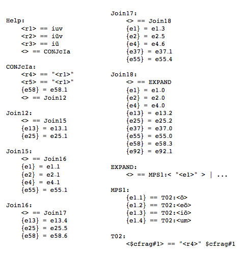
The Help node introduces the three stems required by conjugation cIa. It refers all other requests to the CONJcIa node, which refers the remaining stems to the first stem. It also provisions the version of distillation e58 to have variant 1. It refers other requests to a chain of grouping nodes, here shown as Join12, Join15, Join17, and Join18, each of which provisions some distillations and hands of other requests to the next node in the chain. Finally, node Join18 refers all morphological queries to EXPAND. This node, of which we show only a small piece, combines the result of referring to nodes MPS1 through MPS92, for each one looking up the appropriate exponence. MPS1, which generates the present indicative active first person singular form, invokes node T02 with a parameter that depends on the value of the e1 distillation. Finally, the T02 node looks up the appropriate stem (in this case, stem 4) and combines it with the given ending.
Table 9 shows some of the output that KATR generates for this theory. We use such output to verify that we have correctly captured the original paradigm in our chart of
Table 2.
| iuvō |
iuvās |
iuvat |
iuvāmus |
iuvātis |
iuvant |
| laudō |
laudās |
laudat |
laudāmus |
laudātis |
laudant |
| moneō |
monēs |
monet |
monēmus |
monētis |
monent |
| dūco |
dūcis |
dūcit |
dūcimus |
dūcitis |
dūcunt |
| sum |
es |
est |
sumus |
estis |
sunt |
Table 9.
Output of automatically generated KATR theory (fragment)
Conclusions
This exercise demonstrates that both the realizational and the implicative approaches to defining language morphology lead to effective descriptions, as evidenced by the KATR theories they produce. An advantage of the realizational approach is that it allows us to apply language-specific knowledge and insight to create a default inheritance hierarchy that captures the morphological structure of the language, with slots pertaining to different morphosyntactic properties. However, as we have noted elsewhere [
Finkel 2007b] writing KATR specifications requires considerable effort. Early choices color the structure of the resulting theory, and the author must often discard attempts and rethink how to represent the target morphology. We have built KATR theories for verbs in Hebrew, Slovak, Polish, Spanish, and Lingala (a Bantu language of the Congo), as well as for parts of Hungarian, Sanskrit, and Pali.
The implicative approach is much more automatic. One still needs to manually construct the initial paradigm, decide how many stems are needed (for Latin, we use five; for French, we use 15), and abstract as much information as possible into the templates for each MPS. After that, we can use automatic methods that reduce the paradigm chart to its essence, group conjugations, and generate an effective KATR theory. These steps take only a few seconds to complete (on a 1.8GHz Intel Pentium running Linux, only one second). It is a simple (albeit tedious) matter to verify that all the forms the KATR theory generates are accurate. The KATR theory itself is fairly compact, taking advantage of grouping. However, it is about twice the size of the hand-built theory (measured in characters). More important, it doesn't clearly delineate the slots of the exponences. It is therefore somewhat less satisfying, somewhat less informative, than the KATR theory we build manually following the realizational approach. We have applied the implicative approach to French (both as spelled and as pronounced), Hebrew, and Yiddish, as well as some lesser-known languages, such as Comaltepec Chinantec (Oto-Manguean, spoken in Oaxaca, Mexico), Fur (Nilo-Saharan, in Darfur), and Sora (Austro-Asiatic, India).
The implicative approach also has the advantage that it allows us to analyze the principal parts of the language based solely on the exponences in the paradigm chart. We have taken advantage of that ability elsewhere to characterize languages based on properties of their principal parts [
Finkel 2007a]. For example, Latin, along with Sanskrit, but in strong contradistinction to Comaltepec Chinantec, has a very orthogonal set of principal parts: Each principal part tends to govern a disjoint set of MPSs.
As Latin developed into the Romance languages, its scheme of conjugations and principal parts evolved. Initial investigation of French, following the same implicative approach as that shown here for Latin, shows that 9 static principal parts are needed to distinguish the 67 distinct conjugations. Ignoring spelling and considering only pronunciation, we have been able to reduce this total to 7 principal parts distinguishing 35 conjugations. This investigation continues.
Acknowledgments
We would like to thank Lei Shen and Suresh Thesayi, who were instrumental in implementing our Java™ version of KATR. Nancy Snoke assisted in implementing our Perl/Prolog version.
This work was partially supported by the National Science Foundation under Grants IIS-0097278 and IIS-0325063 and by the University of Kentucky Center for Computational Science. Any opinions, findings, conclusions or recommendations expressed in this material are those of the authors and do not necessarily reflect the views of the funding agencies.
Glossary
-
Cell: A position in a full table of word forms, where the row is the inflection class (such as conjugation 1), and the column represents a set of morphosyntactic properties (such as first person singular present indicative active).
-
Desinence: An inflectional ending, usually added to a stem according to its syntactic context. For example, amat
“he/she loves” has the desinence -t.
-
Diacritic: A marker of a particular morphophonological property. For example, the fact that a verb is in conjugation 4 is a diacritic.
-
Exponence: The contents of a cell for a given lexeme, such as amat.
-
Morphophoneme: A phonological unit whose phonemic expression depends on its context. For example in our Latin KATR theory, we use I as the phonological unit in conjugation 3 (i-stem) that is either expressed as the phoneme i (as in capiō
“I grab”), as the phoneme e (before r, as in capere
“to grab”), or disappears entirely (such as before ī, as in cēpī
“I have grabbed”).
-
Node: A set of rules in a KATR theory to which a query is directed. The particular rule to apply depends on the query. Some nodes refer to others, leading to a hierarchical node structure.
-
Sandhi: Rules of euphony or spelling. For example ēō is pronounced eō, as in videō
“I see,” and cs is spelled x, as in dūxī
“I have led.”
Works Cited
Anderson 1992 Anderson, S. R. 1992 Amorphous morphology, Cambridge University Press.
Blevins 2005 Blevins, J. P. 2005 “Word-based Declensions in Estonian,” in G. Booij & J. van Marle (eds.), Yearbook of Morphology 2005, Springer, Dordrecht, pp. 1–25.
Blevins 2006 Blevins, J. P. 2006 “Word-based Morphology,”
Journal of Linguistics 42: 531– 573.
Corbett 1993 Corbett, G. G. & Fraser, N. M. 1993
“Network Morphology: A DATR Account of Russian Nominal Inflection,”
Journal of Linguistics 29: 113– 142.
Evans 1989 Evans, R. & Gazdar, G. 1989 “Inference in DATR, Proceedings of the Fourth Conference of the European Chapter of the Association for Computational Linguistics,” Manchester, pp. 66–71.
Finkel 2002 Finkel, R., Shen, L., Stump, G. &
Thesayi, S. 2002 “KATR: A Set-based Extension of DATR,” Technical Report 346-02, University of Kentucky Department of Computer Science, Lexington, KY.
ftp://ftp.cs.uky.edu/cs/techreports/346-02.pdf.
Finkel 2007a Finkel, R. A. & Stump, G. T.
(2007a). “Principal Parts and Morphological Typology,”
Morphology 17: 39–75.
Finkel 2007b Finkel, R. & Stump, G. (2007b).
“A Default Inheritance Hierarchy for Computing Hebrew Verb Morphology,”
Literary and Linguistic Computing 22(2): 117–136. dx.doi.org/10.1093/llc/fqm004.
Finkel 2009 Finkel, R. & Stump, G. 2009
“Principal Parts and Degrees of Paradigmatic Transparency,” in J. P. Blevins & J. Blevins (eds), Analogy in Grammar: Form and Acquisition, Oxford University Press, Oxford.
Matthews 1972 Matthews, P. H. 1972 Inflectional Morphology, Cambridge University Press.
Stump 2001 Stump, G. T. 2001 Inflectional Morphology, Cambridge University Press, Cambridge, England.
Zwicky 1985 Zwicky, A. M. 1985 “How to Describe Inflection,”
Proceedings of the 11th Annual Meeting of the Berkeley Linguistics Society , pp. 372–386.