


Volume 12 Number 1
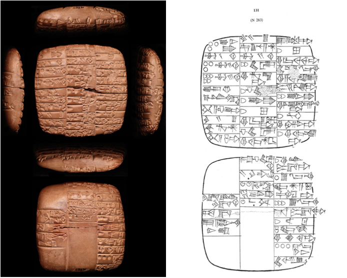
Computational Models for Analyzing Data Collected from Reconstructed Cuneiform Syllabaries
Abstract
This study used three interdependent techniques to help understand the use and distribution of syllabic values of the cuneiform signs during the second half of the third millennium and early second millennium BCE. The results suggest that, during this period, cuneiform syllabaries were variable. That variation can further inform us about the regional, temporal, and dialectical contexts in which they existed. The addition of this research to the wider literature on the early adaptation of cuneiform enhances the field's understanding of how cuneiform syllabic values began to emerge and spread across the ancient Near East, and demonstrates how computational methods of analysis can be applied to research questions in humanities subjects.
1. Background
2. Introduction
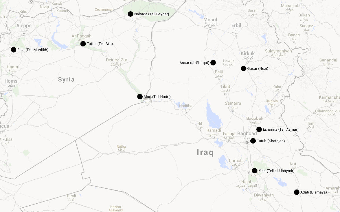
3. Sites Examined
| Site | Region | Period(s) | No. of Texts | Genres (no.) |
| Ebla | Syria | Old Akkadian[7] | ca. 7000 | Lexical[8]; Administrative Letter |
| Mari | Syria | Ur III / Shakkanakku[9] | 463 | Administrative (463) |
| Nabada | Syria | Old Akkadian | 223 | Administrative (222); Legal (1) |
| Tuttul | Syria | Early Old Babylonian[10] | 54 | Administrative (51); Letter (2); Uncertain (1) |
| Adab | S. Mes.[11] | Old Akkadian, Ur III | 1946, 130[12] | Administrative (1854, 102)[13]; Letter (27, 1); Royal/monumental (25, 21); Legal (22, 3); Uncertain (16, 0); Lexical (1, 0); Mathematical (1, 0); School (1, 2) |
| Eshnunna | S. Mes. | Old Akkadian | 261 | Administrative; Uncertain (26); School (8); Letter (6)l Literary (1) |
| Kish | S. Mes. | Old Akkadian | 80 | Administrative (68); Letter (5); Royal/monumental (3); Votive (2); Lexical (1); Literary (1) |
| Tutub | S. Mes. | Old Akkadian | 73 | Administrative (65); Royal/monumental (7); Legal (1) |
| Assur | N. Mes.[14] | Old Akkadian | 20 | Royal/monumental (7); Lexical (6); Administrative (4); School (3) |
| Gasur | N. Mes. | Old Akkadian | 220 | Administrative (190); Lexical (15); Letter (9); Legal (2); School (2); Mathematical (1); Uncertain (1) |
4. Methodology
4.1 Computational methods of analysis: a three-step approach
4.2 Unfiltered and filtered datasets
| Ebla | Mari | Nabada | Tuttul | Adab | Eshnunna | Kish | Tutub | Assur | Gasur |
| 128 | 100 | 70 | 105 | 78 | 60 | 105 | 108 | 6 | 90 |
| Ebla | Mari | Nabada | Tuttul | Adab | Eshnunna | Kish | Tutub | Assur | Gasur |
| 34 | 10 | 4 | 11 | 9 | 1 | 6 | 5 | 0 | 5 |
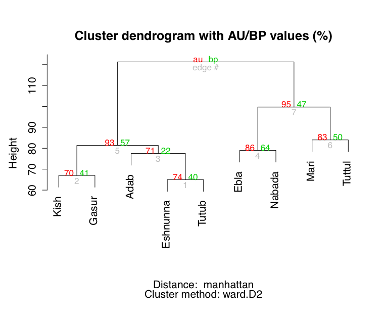
5. Phylogenetic Estimation
5.1 Experimental Method
5.2 Taxa
5.3 Characters
5.4 Program and Settings
5.5 Results


- That the syllabaries exactly mirror the geography of the sites. This would indicate a relationship between the syllabaries that was based purely on geographic proximity of the sites. In other words, this tree would support the conclusion that there was an organic spread of the development and use of syllabic values from site to site.
- That the trees mirror the geography of the sites to a certain extent. This would indicate that geography was perhaps one factor in how similar the syllabaries examined are. In other words, this tree would suggest that sites nearer to each other were more influenced by each other’s syllabaries and sites further away from each other developed “genetic mutations” or independent changes in their syllabaries, but that this was not the sole influencing factor.
- That the trees reflect geography in no way. This would indicate that the differences observed in the syllabaries must be attributed to another cause or causes.


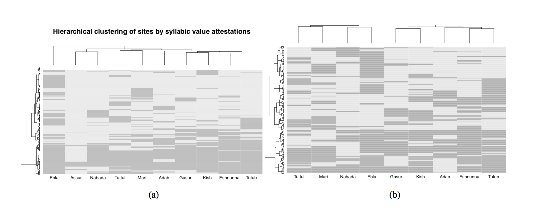
6. Hierarchival Clustering
7. Principal Component Analysis
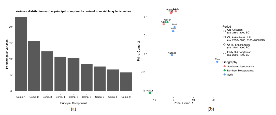
7.1 PCA on the unfiltered dataset: the number of syllabic values attested at each site is driving the observed variation
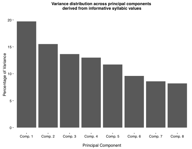
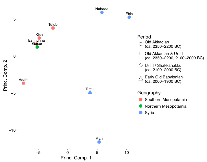
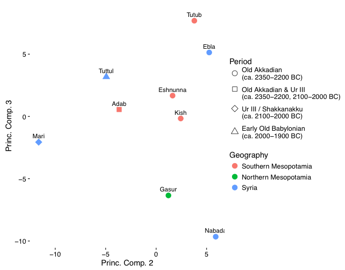
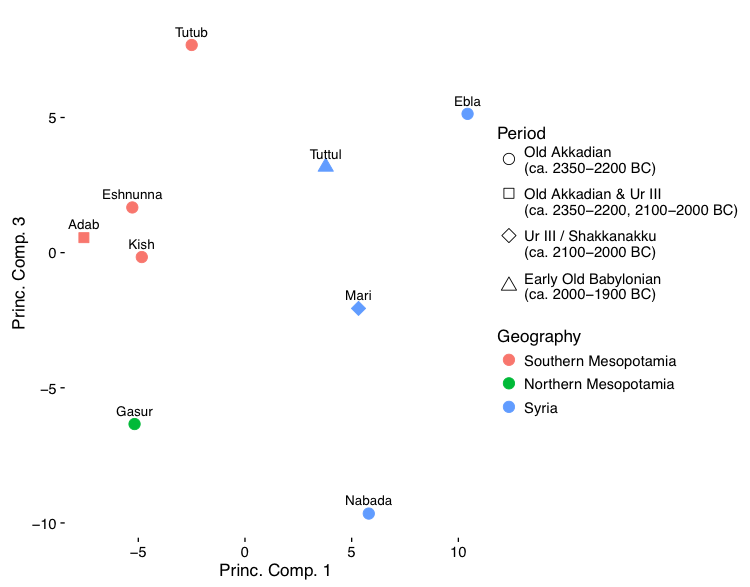
7.2 PCA on the filtered dataset: geographic, temporal, and unknown variation drive the observed variation
7.3 Summary
8. Interpretation of the results of the computational analysis
| Syl. Value | Loading |
| kam | 1.983368897 |
| ḫir | 1.962428466 |
| ba [4] | 1.962428466 |
| qi [2] | 1.962428466 |
| kun | 1.692715905 |
| ag | 1.612331814 |
| tim [x] (DIN) | 1.612331814 |
| tur [2] | 1.545653809 |
| tu [3] | 1.545653809 |
| il | 1.529594896 |
| ku [8] | 1.529594896 |
| dab [6] | 1.431202981 |
| tap [x] | 1.431202981 |
| u [9] | 1.431202981 |
| sum | 1.431202981 |
| kun [3] | 1.431202981 |
| ib [2] | 1.431202981 |
| re [2] | 1.347629658 |
| par [2] | 1.347629658 |
| gur | 1.347629658 |
| qur | 1.347629658 |
| šim | 1.347629658 |
| kak | 1.347629658 |
| iz | 1.347629658 |
| ḫar | 1.347629658 |
| bar | 1.302612779 |
| tar [2] | 1.302612779 |
| nim | 1.203189376 |
| zum | 1.203189376 |
| su [4] | 1.166967631 |
| ši [2] | 1.103759203 |
| Syl. Value | Loading |
| su | 2.722681481 |
| lul | 2.722681481 |
| ib | 2.722681481 |
| bi [2] | 2.348397624 |
| ṣil [2] | 2.348397624 |
| u [3] | 2.348397624 |
| mi | 2.025140491 |
| ar | 2.025140491 |
| sa | 2.000191641 |
| dar | 2.000191641 |
| pum | 1.895816769 |
| pu | 1.80880675 |
| iš [11] | 1.80880675 |
| kab | 1.645361752 |
| se [11] | 1.619356098 |
| re | 1.568075837 |
| un | 1.568075837 |
| qu [2] | 1.56399021 |
| num | 1.484426073 |
| la [2] | 1.388553884 |
| uz | 1.342110283 |
| de [3] | 1.328955355 |
| er | 1.229854594 |
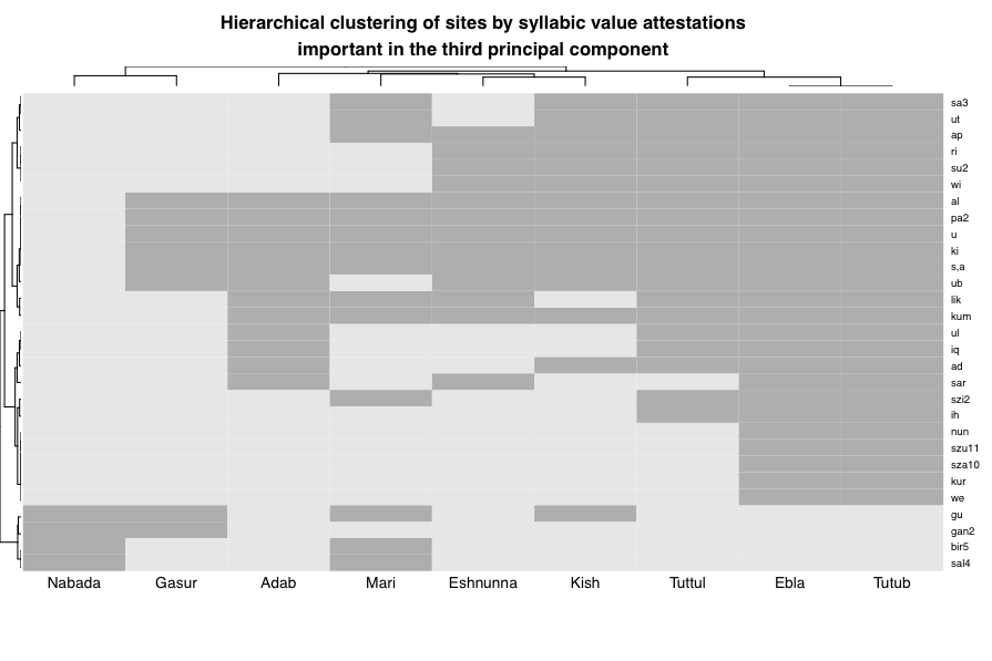
| Syl. Value | Loading |
| gan [2] | 2.65175942 |
| kum | 2.65175942 |
| gu | 2.408786917 |
| su [2] | 2.222928872 |
| ri | 2.222928872 |
| wi | 2.222928872 |
| lik | 2.104672973 |
| iḫ | 2.062260202 |
| iq | 1.986903485 |
| ul | 1.986903485 |
| ad | 1.948006674 |
| ap | 1.922014923 |
| šu [11] | 1.703013331 |
| nun | 1.703013331 |
| ša [10] | 1.703013331 |
| kur | 1.703013331 |
| we | 1.703013331 |
| pa [2] | 1.69043491 |
| al | 1.69043491 |
| u | 1.69043491 |
| ki | 1.69043491 |
| ṣa | 1.69043491 |
| sar | 1.642244435 |
| sal [4] | 1.422929132 |
| bir [5] | 1.422929132 |
| ub | 1.422929132 |
| ši [2] | 1.408110193 |
| ut | 1.375395679 |
| sa [3] | 1.375395679 |
8.1 Geographic variation: the primary explanation of variation in the data
8.2 Temporal variation: the secondary explanation of variation in the data

8.3 Indeterminable variation: the third explanation of variation in the dataset

9. Summary of results
10. Conclusions
10.1 Methodology
10.2 Assyriological Implications
11. Future Applications
11.1 A more comprehensive investigation into third millennium Akkadian
11.2 Applications of this methodology to all East Semitic dialects
- Eblaite (ca. 2350-2250 BC)
- Old Akkadian (ca. 2350-2200 BC)
- Ur III Akkadian (ca. 2100-2000 BC)
- Old Assyrian (ca. 1950-1850 BC)
- Old Babylonian (ca. 2000-1600 BC)
- Middle Assyrian (ca. 1400-1000 BC)
- Middle Babylonian (ca. 1400-1100 BC)
- Neo-Assyrian (ca. 911-612 BC)
- Neo-Babylonian (ca. 626-539 BC)
11.3 Comparing computational methods to find the optimal approach
11.4 Applications to the problem of texts with no known provenance
12. Input Data
12.1 Phylogenetic Estimation
a. Unfiltered data
#NEXUS
Begin taxa;
    Dimensions ntax=10;
    taxlabels
        Ebla
        Mari
        Nabada
        Tuttul
        Adab
        Eshnunna
        Kish
        Tutub
        Assur
        Gasur
    ;
End;
Begin data;
    Dimensions ntax=10 nchar=319;
    Format datatype=standard;
    Matrix
        Ebla  1 0 0 1 1 1 1 1 1 1 1 1 1 0 1 1 1 0 0 1 1 1 0 0 1 1 1 1
        0 0 1 1 0 1 0 0 1 1 1 1 0 0 0 0 1 1 1 1 1 1 1 1 1 1 1 1 1 1 1
        0 1 1 1 1 1 1 1 1 1 1 1 0 1 1 0 1 1 1 0 1 1 1 1 0 1 1 1 1 1 0
        1 1 0 0 0 0 0 1 1 1 1 1 1 0 1 1 0 1 1 1 0 1 0 0 0 0 1 1 1 1 0
        0 1 0 1 1 1 0 0 0 1 0 1 0 1 1 0 1 1 1 0 0 1 1 1 1 0 1 0 0 1 1
        0 0 0 1 1 0 1 1 0 1 1 0 1 0 0 1 1 1 1 0 1 1 1 1 1 1 0 0 1 0 1
        1 0 1 1 0 0 1 1 0 1 1 0 0 0 1 1 0 1 1 1 0 0 0 0 0 1 1 1 1 1 1
        1 1 0 1 1 1 1 1 1 1 0 0 1 0 0 0 1 1 1 1 0 1 1 1 1 1 0 1 0 1 0
        1 1 0 1 0 1 1 1 1 1 0 1 0 0 0 1 1 1 1 1 1 1 1 0 1 1 0 0 1 1 0
        0 0 1 1 0 1 0 1 0 1 0 1 1 0 0 0 0 0 0 1 0 0 1 0 0 1 0 1 1 1 0
        0 1 0 1 1 1 1 1 0 0 0 0

        Mari  0 0 0 0 0 1 1 1 0 0 0 0 0 0 0 0 1 0 1 0 0 0 1 1 0 0 1 1
        0 1 0 0 1 1 0 0 1 0 0 1 0 0 1 1 1 1 0 1 1 0 0 1 0 1 1 1 0 1 1
        1 0 0 0 0 1 1 1 0 0 0 0 1 0 0 0 0 0 0 0 0 1 1 1 0 1 0 0 0 0 1
        0 0 0 0 0 0 1 0 1 1 1 1 1 1 1 1 1 1 1 1 0 0 1 1 0 0 0 0 1 0 0
        0 1 0 1 0 1 1 0 0 1 0 1 0 0 0 0 1 0 0 0 0 0 0 0 1 1 0 0 0 1 0
        0 0 0 1 0 0 0 1 0 0 1 0 1 0 0 1 1 1 1 0 1 0 1 1 1 0 1 0 1 0 1
        0 0 1 1 1 0 1 1 1 1 1 0 0 0 0 1 0 1 0 1 1 0 1 1 0 1 0 1 1 0 1
        0 1 0 0 1 1 0 0 0 1 1 0 0 1 1 0 1 0 0 1 0 0 0 1 0 0 0 1 0 1 0
        0 0 0 1 0 1 1 0 1 0 1 0 1 0 1 0 0 0 1 1 0 0 0 0 1 1 0 1 0 1 1
        1 1 0 1 1 0 0 1 1 1 0 1 0 0 0 0 1 0 0 1 1 1 1 0 0 1 1 0 0 1 0
        1 1 0 1 1 1 1 0 0 0 0 0

        Nabada  1 0 0 0 0 1 0 1 0 0 1 0 0 0 0 0 1 1 1 0 1 0 0 0 1 1 1
        0 0 0 1 0 0 1 0 0 1 0 0 1 0 0 0 1 1 1 0 1 1 1 0 0 0 1 0 1 1 1
        0 1 0 1 0 0 1 0 0 0 0 0 0 0 0 0 0 0 1 0 0 0 1 0 0 0 1 0 0 0 0
        0 1 0 1 0 0 0 0 1 1 0 0 1 0 0 1 1 0 1 1 0 0 0 0 0 0 0 1 1 1 0
        0 0 1 0 1 0 1 0 0 0 1 0 1 0 1 1 0 1 1 1 0 1 0 0 0 0 0 1 0 0 1
        1 0 0 0 1 1 0 1 0 0 0 1 0 1 0 0 0 0 0 1 0 1 0 1 0 1 0 0 0 0 0
        0 0 0 0 1 0 0 1 0 0 1 1 0 0 0 0 0 0 1 0 1 0 1 0 0 0 1 0 1 1 0
        1 0 0 0 0 1 1 1 0 0 1 0 1 0 0 0 0 0 0 1 0 0 0 0 1 0 0 0 1 0 0
        0 0 0 0 1 0 0 0 0 0 1 0 0 0 0 0 0 1 0 1 1 1 1 0 0 1 0 0 0 0 0
        0 0 0 0 1 0 1 1 1 0 0 0 1 0 1 0 0 0 0 0 0 0 1 0 0 0 1 0 0 0 0
        0 0 1 0 1 0 0 1 1 0 0 0 0

        Tuttul  1 0 0 0 0 1 1 1 1 1 0 0 1 1 1 0 1 0 1 1 0 0 1 1 0 0 1
        0 0 0 1 0 0 1 1 0 1 0 0 1 1 1 0 0 1 1 0 1 1 0 0 0 0 1 0 1 1 1
        0 0 0 1 0 1 1 1 0 0 0 0 1 1 0 0 1 0 0 0 0 0 1 1 0 1 1 0 0 0 0
        0 1 0 0 0 0 0 0 1 1 0 0 1 1 0 1 0 0 0 1 1 0 0 0 0 0 1 0 0 1 0
        0 1 1 1 1 1 1 0 0 0 1 0 0 0 0 0 1 1 0 0 0 0 0 0 0 1 0 0 0 0 1
        1 0 0 0 1 1 0 0 0 0 0 1 0 1 1 1 0 0 1 1 0 1 0 1 0 0 1 0 0 0 0
        1 1 1 0 1 1 0 1 1 0 1 1 0 0 1 1 0 0 1 0 1 0 0 0 0 0 1 0 1 1 0
        1 0 0 0 0 1 1 0 0 0 1 1 0 0 0 0 1 0 0 1 1 0 0 1 0 0 0 1 1 0 1
        1 1 1 0 1 1 0 0 0 1 1 1 0 0 0 1 0 0 1 0 0 1 0 1 1 1 1 1 1 0 1
        0 0 1 0 1 1 0 1 1 1 1 0 1 0 0 0 0 0 0 0 0 0 0 0 0 1 0 0 0 1 1
        0 0 1 0 1 1 1 1 0 0 0 0 0

        Adab  1 1 1 0 0 1 1 1 0 0 0 0 0 0 0 0 1 0 0 0 1 0 0 1 1 1 1 0
        0 0 1 0 0 0 1 1 0 0 0 1 0 0 0 0 0 1 0 0 1 1 0 0 0 0 0 1 0 1 0
        0 0 0 1 1 0 0 0 0 0 0 0 0 0 0 1 0 0 0 0 0 0 0 0 0 1 0 0 0 0 0
        0 0 0 0 0 1 0 0 0 0 0 1 0 1 1 0 0 0 0 0 0 0 0 0 0 0 0 0 1 0 1
        0 1 0 1 1 1 0 0 1 1 1 0 0 0 0 0 1 1 1 1 0 0 0 0 1 0 0 1 1 0 1
        1 1 0 1 0 0 0 1 0 0 1 0 1 0 1 0 0 1 1 0 1 0 1 1 0 0 1 0 0 0 1
        1 0 0 1 0 1 0 1 1 1 1 0 0 1 0 1 1 1 1 1 1 0 0 1 0 1 0 1 1 0 1
        0 1 0 1 1 1 0 0 0 1 1 0 0 0 0 0 0 0 0 0 0 0 0 1 1 0 0 1 0 1 0
        0 0 1 1 0 0 1 0 1 1 0 0 0 0 0 1 0 1 0 1 1 1 0 0 0 1 1 0 0 0 0
        0 1 0 1 0 0 0 1 1 1 0 1 0 0 0 0 0 0 0 0 0 0 1 1 0 1 1 0 1 1 0
        0 1 1 0 1 0 0 0 0 0 0 1

        Eshnunna  0 0 0 0 0 1 1 0 1 0 1 0 0 0 0 0 1 0 1 0 0 0 0 0 1 1
        1 0 1 1 1 0 1 1 1 1 1 0 0 1 0 0 0 0 1 1 0 1 1 1 0 0 0 1 0 1 0
        1 0 0 0 0 1 0 1 1 0 0 1 0 1 0 0 0 0 0 1 0 0 0 1 0 1 0 1 0 0 0
        0 0 1 0 0 0 0 1 0 1 1 0 0 1 0 1 1 0 0 1 0 1 0 0 0 0 0 0 0 0 1
        0 0 0 1 0 0 0 1 0 1 1 1 0 0 0 0 0 0 1 1 1 0 0 0 0 0 1 0 0 0 0
        1 1 1 0 1 1 1 0 0 1 0 0 1 0 1 0 1 0 0 1 1 0 1 0 1 1 0 1 1 1 0
        0 1 1 0 1 1 0 0 1 1 1 1 1 0 0 1 0 1 0 1 1 0 1 0 0 0 0 1 1 1 1
        0 1 1 1 0 1 1 1 1 0 0 1 1 1 0 0 0 0 1 0 1 0 0 0 1 1 0 0 0 1 0
        1 0 0 0 1 1 0 0 1 0 1 1 0 0 1 1 1 1 0 0 1 1 1 1 0 0 1 1 1 1 0
        0 0 1 0 0 1 0 1 1 1 1 0 1 1 0 0 1 0 0 1 0 0 1 0 0 0 1 1 1 0 1
        1 1 0 1 0 1 1 0 1 1 0 0 0 0

        Kish  0 0 0 0 0 1 1 1 1 0 1 0 0 0 0 0 1 0 0 0 0 0 0 1 0 1 1 0
        0 1 1 0 0 1 0 0 1 0 0 1 0 0 0 0 1 1 0 1 1 1 0 0 0 0 0 1 0 1 1
        0 0 1 0 0 1 1 0 1 0 1 1 0 0 0 0 0 0 0 0 0 1 0 1 0 1 0 0 0 0 0
        1 0 0 1 1 1 0 1 0 0 0 1 0 1 1 1 0 1 1 1 0 0 0 0 0 0 0 0 1 0 1
        0 1 0 0 1 1 1 0 0 1 0 0 1 0 0 0 1 1 0 1 0 0 0 0 1 1 0 0 0 0 1
        1 0 1 1 0 0 0 1 0 0 1 1 1 0 0 0 0 1 1 0 1 0 1 0 0 0 0 1 0 1 1
        1 1 0 1 0 0 1 1 1 1 1 1 1 1 1 1 0 1 0 1 0 0 0 1 1 1 0 1 1 0 1
        0 0 0 1 1 1 1 0 0 1 0 1 0 0 0 0 1 0 0 1 0 0 1 0 1 0 0 1 0 1 0
        0 0 1 1 0 0 1 1 1 1 0 1 1 1 0 0 1 0 0 1 1 1 0 0 1 1 1 1 0 0 0
        0 0 0 1 1 1 1 1 1 0 1 1 0 0 1 0 0 1 0 1 0 1 0 1 0 1 1 0 0 0 0
        0 1 0 1 1 1 1 1 1 0 0 0

        Tutub 1 0 0 0 0 1 1 1 1 1 1 1 0 0 0 0 1 0 0 0 0 0 1 0 0 0 1 0
        0 1 1 0 0 1 1 0 1 0 0 1 0 0 0 0 1 1 0 1 1 1 0 0 0 1 0 1 0 1 0
        0 0 1 1 1 1 0 1 0 1 1 1 0 0 0 0 1 1 0 0 0 1 0 1 0 1 0 0 0 0 0
        1 1 0 0 0 1 0 1 1 0 0 1 1 0 1 0 0 1 1 1 1 0 1 0 1 0 0 0 1 0 0
        0 1 0 1 1 1 0 1 0 1 1 0 0 0 0 1 1 1 1 1 0 0 0 0 1 1 0 0 0 0 1
        1 0 1 1 0 0 0 1 1 0 1 0 1 0 0 0 0 1 1 1 1 0 1 1 0 0 1 0 0 0 1
        1 0 0 1 0 0 1 1 1 1 1 0 0 1 0 1 0 1 1 1 1 0 0 1 0 1 0 1 1 0 1
        1 1 0 0 1 1 1 1 0 1 0 1 0 0 0 0 0 0 0 1 1 0 1 1 0 1 0 1 0 0 1
        0 1 0 1 0 0 1 1 1 1 0 0 1 1 0 0 1 1 1 1 1 1 0 1 1 1 1 0 0 0 0
        0 1 0 1 0 1 1 1 0 1 0 1 0 0 1 1 0 1 0 0 0 0 0 1 1 1 1 0 0 1 1
        0 1 0 1 1 1 1 0 0 0 0 0

        Assur 0 0 0 0 0 1 0 1 0 0 1 0 0 0 0 0 1 0 0 0 0 0 0 0 0 0 1 0
        0 0 1 0 0 1 0 0 0 0 0 1 0 0 0 0 0 1 0 1 1 0 0 0 0 0 0 1 0 0 0
        0 0 1 0 0 0 0 0 0 0 0 0 0 0 0 0 0 0 0 0 0 0 0 0 0 0 0 0 0 0 0
        1 0 0 0 0 0 0 0 0 0 0 0 0 0 0 0 0 0 0 0 0 0 0 0 0 0 0 0 0 0 0
        0 1 0 0 0 0 0 0 0 0 0 0 0 0 0 0 0 0 0 0 0 0 0 0 0 0 0 0 0 0 0
        0 0 0 1 0 0 0 1 0 0 1 0 0 0 0 0 0 1 1 0 0 0 0 0 0 0 0 0 0 0 0
        0 0 0 0 0 0 0 1 0 0 0 0 0 0 0 0 0 0 0 0 0 0 0 0 0 0 0 0 0 0 1
        0 0 0 0 0 0 0 0 0 0 0 0 0 0 0 0 0 0 0 0 0 0 0 0 0 0 0 0 0 0 0
        0 0 0 0 0 0 0 0 0 0 0 0 0 0 0 0 0 0 0 0 0 0 0 0 0 0 0 0 0 0 0
        0 0 0 0 0 0 0 0 0 0 0 0 0 0 0 0 0 1 0 0 0 0 0 0 0 0 0 0 0 0 0
        0 1 0 0 0 0 0 0 0 0 0 0

        Gasur 0 0 0 1 0 1 1 1 0 1 1 0 0 0 0 0 1 0 0 0 0 0 0 0 0 1 1 0
        0 1 1 0 0 1 1 0 1 0 0 1 0 0 0 0 1 1 0 1 1 1 0 1 0 0 0 1 0 1 1
        0 0 0 1 0 1 1 0 0 1 0 0 1 0 0 0 0 0 0 1 0 1 0 0 0 1 0 0 0 0 0
        1 0 1 0 1 0 0 1 0 0 0 1 0 1 1 0 0 1 1 0 0 0 1 0 0 0 0 0 1 0 0
        0 1 0 0 0 1 0 1 0 1 0 0 0 0 0 0 1 1 1 0 0 0 0 0 0 0 0 0 0 0 0
        0 0 0 1 0 0 0 1 1 0 1 0 1 0 0 0 0 1 1 0 1 0 1 1 0 0 0 1 0 1 1
        1 1 0 1 1 0 0 1 0 1 0 0 0 0 0 1 0 1 0 1 0 0 0 1 1 1 0 1 1 0 1
        1 0 1 0 1 1 1 0 0 1 1 1 0 0 0 0 1 0 1 0 0 0 0 1 0 0 0 1 1 1 1
        1 0 1 1 0 0 1 0 1 1 0 0 0 1 0 1 0 0 1 0 1 1 0 0 0 1 1 0 0 0 0
        0 1 0 1 1 1 0 1 0 1 1 1 0 0 1 0 1 0 0 0 0 1 0 1 0 1 0 0 1 0 0
        0 1 0 1 1 0 1 1 0 1 1 0

        ;
End;
b. Filtered data
\#NEXUS
Begin taxa;
    Dimensions ntax=9;
    taxlabels
        Ebla
        Mari
        Nabada
        Tuttul
        Adab
        Eshnunna
        Kish
        Tutub
        Gasur
    ;
End;
Begin data;
    Dimensions ntax=9 nchar=188;
    Format datatype=standard;
    Matrix
        Ebla  1 1 1 1 1 1 1 1 1 0 1 1 0 0 1 1 1 0 0 0 0 1 0 1 1 1 1 1
        1 1 0 1 1 1 1 1 1 1 1 1 1 0 0 1 1 1 1 1 1 1 0 0 0 1 1 1 1 1 0
        1 1 1 1 0 1 1 0 1 1 0 0 0 0 1 1 1 0 1 1 0 1 0 1 1 1 0 0 1 1 1
        0 0 1 1 0 1 1 0 0 1 0 1 1 0 1 0 1 0 1 0 1 1 1 1 0 0 0 1 1 1 1
        1 1 0 0 1 1 1 1 1 1 1 1 0 1 1 0 1 1 1 1 1 0 1 0 0 0 1 1 1 1 1
        1 1 1 0 1 1 0 0 1 0 0 0 1 0 0 1 0 0 0 0 1 0 0 1 0 0 1 0 1 1 0
        1 1 1 1 1

        Mari  0 0 1 0 0 0 0 0 0 1 0 0 1 1 0 0 1 1 1 0 0 1 1 1 0 1 1 1
        0 1 1 0 0 0 1 1 1 0 0 0 0 1 0 0 0 1 1 1 0 0 0 0 0 0 1 1 1 1 1
        1 1 1 1 1 0 0 0 1 0 1 0 0 0 1 0 0 0 0 0 0 1 1 0 1 0 0 0 0 0 1
        0 0 1 1 1 1 0 1 0 1 0 1 0 0 1 1 1 1 1 0 0 1 0 1 1 1 0 0 0 1 0
        0 0 1 0 1 0 1 0 1 0 0 1 0 0 0 0 1 1 0 1 0 1 0 1 0 1 0 0 0 1 1
        0 0 0 0 1 1 0 1 1 1 1 1 0 0 1 1 0 0 1 0 1 1 1 1 0 0 1 1 0 1 0
        1 1 1 1 0

        Nabada  1 0 0 0 0 1 0 0 0 1 0 1 0 0 1 1 0 0 0 0 0 1 1 1 0 0 1
        0 1 0 1 1 0 0 1 0 0 0 0 0 0 0 0 0 1 1 0 0 1 0 1 0 0 1 1 0 0 0
        0 1 1 1 0 0 1 1 0 1 0 0 0 0 0 1 1 1 0 1 1 0 0 0 1 1 1 0 0 1 1
        0 0 0 0 0 0 1 0 0 0 0 0 0 0 0 0 0 1 0 1 0 0 0 0 1 0 0 0 0 0 0
        0 1 0 0 1 0 1 0 0 1 0 0 0 0 0 0 0 0 0 0 0 1 0 0 0 0 0 0 1 0 1
        1 1 1 0 0 1 0 0 0 0 0 0 0 1 1 0 0 0 0 0 0 0 0 1 0 0 0 1 0 0 0
        0 1 0 0 1 1

        Tuttul  1 0 1 1 1 0 0 1 1 1 1 0 1 1 0 0 0 0 0 1 0 1 0 1 0 0 1
        0 1 0 0 1 0 1 1 1 0 0 0 0 1 1 1 0 0 1 1 0 1 0 0 0 0 1 1 0 0 1
        0 0 0 1 1 0 0 0 0 1 1 0 0 0 0 0 0 0 1 0 0 0 1 0 0 1 1 0 0 1 0
        0 0 1 0 0 1 0 1 0 0 0 0 1 1 1 0 1 1 0 1 1 1 0 0 1 0 0 0 0 0 0
        0 0 0 1 0 0 1 1 1 0 0 0 1 1 1 1 0 0 0 0 1 1 1 0 0 0 1 0 0 1 0
        0 1 0 1 1 1 1 1 1 1 0 1 1 0 1 1 1 0 0 0 0 0 0 0 0 0 1 0 0 1 1
        0 1 1 1 1 0

        Adab  1 0 1 0 0 0 0 0 0 0 0 1 0 1 1 1 0 0 0 1 1 0 0 0 1 0 0 0
        0 0 0 0 1 1 0 0 0 0 0 0 0 0 1 0 0 0 0 0 0 0 0 0 1 0 0 0 0 0 1
        0 0 0 0 0 0 0 1 1 1 0 0 1 1 0 0 0 0 1 1 1 1 0 0 0 1 1 0 0 0 1
        0 1 0 0 1 0 0 1 0 0 0 1 1 0 0 0 0 1 1 1 0 1 1 1 1 1 0 0 0 1 1
        0 0 1 0 0 0 0 0 1 1 0 1 0 0 0 1 0 1 0 1 1 0 0 0 0 0 1 0 1 0 1
        1 1 0 0 0 1 1 0 0 0 1 0 0 0 1 1 0 0 0 0 0 0 0 1 1 0 1 1 1 1 0
        0 1 0 0 0

        Eshnunna  0 0 1 1 0 1 0 0 0 1 0 0 0 0 1 1 0 1 1 1 1 1 0 1 1 0
        1 0 0 0 0 0 1 0 1 1 0 0 1 0 1 0 0 0 1 1 0 1 1 0 0 0 1 1 1 0 0
        0 1 0 1 0 1 0 0 0 0 0 0 0 1 1 0 0 0 0 0 1 1 0 1 0 0 1 1 1 1 1
        0 1 0 1 0 0 1 0 1 1 1 0 0 1 1 0 1 0 1 1 1 1 0 1 1 0 1 0 0 1 1
        1 1 1 0 1 1 1 1 0 1 1 0 0 1 0 0 0 1 0 1 0 1 1 0 0 1 1 1 1 0 0
        1 1 1 1 0 0 1 1 1 1 0 1 0 0 1 1 1 0 1 1 0 1 0 1 0 0 0 1 1 1 1
        1 1 1 1 0 1 1

        Kish  0 0 1 1 0 1 0 0 0 0 0 0 0 1 0 1 0 1 0 0 0 1 0 1 1 0 0 0
        0 1 0 1 0 0 1 1 0 1 0 1 1 0 0 0 0 1 0 1 1 0 0 1 1 1 0 0 0 0 1
        1 1 1 1 0 0 0 1 0 1 1 0 0 0 0 0 0 0 1 0 1 1 1 0 0 1 1 1 0 0 1
        0 0 0 0 0 0 0 0 1 0 1 1 1 1 0 0 1 1 1 1 1 1 0 1 0 1 1 0 0 0 1
        1 0 0 1 1 0 1 1 0 1 0 1 0 0 0 1 0 1 1 1 1 0 1 1 1 0 0 1 0 0 1
        1 1 0 0 1 1 1 1 0 0 0 1 1 1 1 0 1 1 0 1 1 0 1 0 1 0 1 1 0 0 0
        1 1 1 1 1

        Tutub 1 0 1 1 1 1 1 0 0 0 0 0 1 0 0 0 0 1 0 1 0 1 0 1 1 0 1 0
        0 0 0 1 1 1 1 0 1 0 1 1 1 0 0 1 1 1 0 1 1 1 0 0 1 1 1 0 0 1 0
        0 1 1 1 1 0 0 0 1 1 0 1 0 1 0 0 0 1 1 1 1 1 1 0 0 1 1 1 0 0 1
        1 0 0 0 1 0 0 1 0 0 0 1 1 0 0 0 1 1 1 1 0 1 1 1 1 1 0 0 1 1 0
        1 1 0 1 0 0 1 1 1 0 1 0 1 0 1 0 0 1 1 1 1 0 0 1 1 0 0 1 1 1 1
        1 1 0 1 1 1 1 0 0 0 1 0 1 1 0 1 0 1 0 1 0 0 0 0 1 1 1 1 0 1 1
        1 1 1 1 0

        Gasur 0 1 1 0 1 1 0 0 0 0 0 0 0 0 0 1 0 1 0 1 0 1 0 1 1 1 0 0
        0 1 0 0 1 0 1 1 0 0 1 0 0 1 0 0 0 1 0 0 1 0 1 1 0 1 0 0 0 0 1
        0 1 1 0 1 0 0 0 0 0 0 1 0 0 0 0 0 0 1 1 0 0 0 0 0 0 0 0 0 0 1
        1 0 0 0 1 0 0 0 1 0 1 1 1 1 0 1 0 0 0 0 0 1 0 1 0 1 1 0 1 0 0
        1 0 1 1 1 1 0 0 1 0 0 1 1 1 0 1 0 1 0 1 1 0 0 0 1 0 1 0 0 1 0
        1 1 0 0 0 1 1 0 0 0 1 1 1 0 0 1 1 1 1 0 0 0 1 0 1 0 1 0 1 0 0
        1 1 0 1 1

    ;
End;
\pagebreak
12.2 RStudio
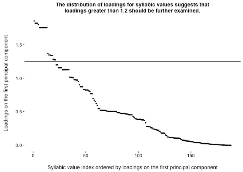
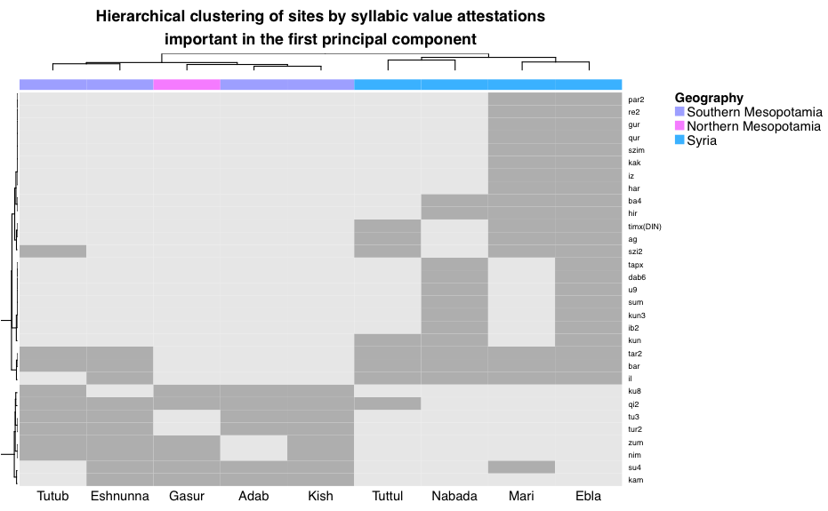
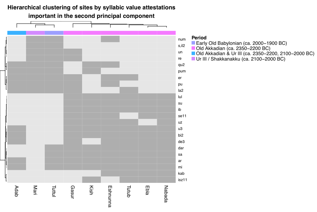
    \begin{verbatim}

    library("NMF")
    library("FactoMineR")
    library("data.table")
    library("ggplot2")
    library("cowplot")
    library("ggdendro")
    library("pvclust")
    #data.df<-data.frame(syl_matrix_forR_090416)[1:319,5:14]
    data.df<-data.frame(syl_matrix_forR_090416)[1:319,4:14]
    rownames(data.df)<-data.df$Sign.Value
    data.df<-data.df[,2:11]
    data.df<-data.df[rowSums(data.df)>0,]

    #unfiltered w/ Assur
    colnames(data.df)<-gsub("Esznunna","Eshnunna",colnames(data.df))
    rclust<-hclust(dist(data.df,method="manhattan"), method="ward.D2")
    cclust<-hclust(dist(t(data.df),method="manhattan"), method="ward.D2")
    aheatmap(data.df,color='grey:2', Rowv=rclust,breaks=c(-0.05,0.5,1.05),
    labRow=NULL,main="Hierarchical clustering of sites by syllabic value
    attestations \n", legend=FALSE, fontsize=14, cexCol = 0.8)

    #unfiltered data w/ Assur
    forpca<-t(data.df)
    answer<-PCA(forpca,ncp=10,graph=FALSE)
    pc.eig.df<-data.frame(answer$eig)
    ggplot(data=pc.eig.df[c(1:9),], aes(x=gsub("comp","Comp.",
        rownames(pc.eig.df[c(1:9),])), y=percentage.of.variance)) +
    geom_bar(stat="identity" +xlab("\nPrincipal Component")
        +ylab("Percentage of Variance") +ggtitle("Variance distribution
        across principal components derived from viable syllabic values")
        coord.rs.df<-data.frame(answer$ind$coord)
        gsub("Esznunna","E?nunna",row.names(coord.rs.df))
        Geography<-factor(c("Syria", "Syria", "Syria", "Syria", "Southern
        Mesopotamia", "Southern Mesopotamia", "Southern Mesopotamia",
        "Southern Mesopotamia", "Northern Mesopotamia", "Northern Mesopotamia"),
        levels=c("Southern Mesopotamia", "Northern Mesopotamia", "Syria"))
        Period<-factor(c("Old Akkadian\n(ca. 2350-2200 BC)", "\nUr III/
        Shakkanakku\n(ca. 2100-2000 BC)", "Old Akkadian\n(ca. 2350-2200 BC)",
        "\nEarly Old Babylonian\n(ca. 2000-1900 BC)\n", "\nOld Akkadian & Ur
        III\n(ca. 2350-2200, 2100-2000 BC)", "Old Akkadian \n(ca. 2350-2200 BC)",
        "Old Akkadian\n(ca. 2350-2200 BC)", "Old Akkadian\n(ca. 2350-2200 BC)", "Old
        Akkadian\n(ca. 2350-2200 BC)", "Old Akkadian\n(ca. 2350-2200 BC)"),
        levels=c("Old Akkadian\n(ca. 2350-2200 BC)", "\nOld Akkadian & Ur
        III\n(ca. 2350-2200, 2100-2000 BC)", "\nUr III / Shakkanakku \n(ca.
        2100-2000 BC)", "\n Early Old Babylonian \n(ca. 2000-1900 BC)\n"))
    ggplot(data=coord.rs.df, aes(x=Dim.1, y=Dim.2))+geom_point(aes(shape=Period,
        fill=Geography, color=Geography),size=4)+scale_shape_manual
        (values=c(21,22,23,24))+xlab("Princ. Comp. 1")+ylab("Princ. Comp. 2")
        +geom_text(label=gsub("Esznunna","E?nunna", row.names(coord.rs.df)),
        nudge_y=0.7)

    #filtering out hapax signs and allsites signs
    data2.df<-data.df[rowSums(data.df)>1 & rowSums(data.df)<9,-9]
    colnames(data2.df)<-gsub("Esznunna","Eshnunna",colnames(data2.df))
    colnames(data.df)<-gsub("Esznunna","Eshnunna",colnames(data.df))

    #convert table into final table for thesis for hapax signs
    data.onesite.df<-data.df[rowSums(data.df)==1,]
    data.onesite.df$Site<-"DUMMY"
    data.onesite.df[data.onesite.df$Ebla==1,]$Site<-"Ebla"
    data.onesite.df[data.onesite.df$Mari==1,]$Site<-"Mari"
    data.onesite.df[data.onesite.df$Nabada==1,]$Site<-"Nabada"
    data.onesite.df[data.onesite.df$Tuttul==1,]$Site<-"Tuttul"
    data.onesite.df[data.onesite.df$Adab==1,]$Site<-"Adab"
    data.onesite.df[data.onesite.df$E?nunna==1,]$Site<-"E?nunna"
    data.onesite.df[data.onesite.df$Kish==1,]$Site<-"Kish"
    data.onesite.df[data.onesite.df$Tutub==1,]$Site<-"Tutub"
    #data.onesite.df[data.onesite.df$Assur==1,]$Site<-"Assur"
    data.onesite.df[data.onesite.df$Gasur==1,]$Site<-"Gasur"
    final.onesite.dt<-data.table(data.onesite.df,
    final.onesite.dt<-final.onesite.dt[order(Site)]
    keep.rownames=TRUE)[,.(rn, Site)] write.table(final.onesite.dt,
    file="hapax_signs.xls", quote=FALSE, sep="\t", row.names=FALSE)

    #table of signs that occur at all sites
    data.allsites.df<-data.df[rowSums(data.df[,-9])==9,-9]
    write.table(rownames(data.allsites.df), file="allsites_signs.xls",
        quote=FALSE, sep="\t", row.names=FALSE)

    #table of filtered data
    write.table(rownames(data2.df),file="data_filtered.xls", quote=FALSE,
        sep="\t", row.names=TRUE, col.names=TRUE)
    write.table(data2.df,file="data_filtered.xls",sep="\t")

    #hierarchical clustering
    colnames(data2.df)<-gsub("Esznunna","Eshnunna",colnames(data2.df))
    rclust<-hclust(dist(data2.df,method="manhattan"), method="ward.D2")
    cclust<-hclust(dist(t(data2.df),method="manhattan"), method="ward.D2")
    aheatmap(data2.df,color='grey:2', Rowv=rclust,breaks=c(-0.05,0.5,1.05),
        labRow=NULL, legend=FALSE, fontsize=14, cexCol = 0.8)
    result <-pvclust(data2.df, method.dist="manhattan",
        method.hclust="ward.D2", nboot=10000)
    plot(result)

    #PCA
    colnames(data2.df)<-gsub("E?nunna","Eshnunna",colnames(data2.df))
    forpca<-t(data2.df)
    answer<-PCA(forpca,ncp=3,graph=FALSE)
    pc.eig.df<-data.frame(answer$eig)
    ggplot(data=pc.eig.df[c(1:8),], aes(x=gsub("comp","Comp.",
        rownames(pc.eig.df[c(1:8),])), y=percentage.of.variance)) +
        geom_bar(stat="identity")+xlab("\nPrincipal Component") +
        ylab("Percentage of Variance")+ggtitle("Variance distribution across
        principal components \n derived from informative syllabic values \n")
    coord.rs.df<-data.frame(answer$ind$coord)
    #meta.pca.df<-meta.df[rownames(coord.rs.df),]

    #PC1
    gsub("Esznunna","Eshnunna", row.names(coord.rs.df))
    Geography<-factor(c("Syria", "Syria", "Syria", "Syria", "Southern
        Mesopotamia", "Southern Mesopotamia", "Southern Mesopotamia", "Southern
        Mesopotamia", "Northern Mesopotamia"), levels=c("Southern Mesopotamia",
        "Northern Mesopotamia", "Syria"))
    Period<-factor(c("Old Akkadian\n(ca. 2350-2200 BC)", "\nUr III /
        Shakkanakku \n(ca. 2100-2000 BC)", "Old Akkadian\n(ca. 2350-2200 BC)",
        "\nEarly Old Babylonian\n(ca. 2000-1900 BC)\n", "\nOld Akkadian &
        Ur III \n(ca. 2350-2200, 2100-2000 BC)", "Old Akkadian\n(ca. 2350-2200 BC)",
        "Old Akkadian \n(ca. 2350-2200 BC)", "Old Akkadian\n(ca. 2350-2200 BC)",
        "Old Akkadian\n(ca. 2350-2200 BC)"), levels=c("Old Akkadian \n(ca. 2350-2200 BC)",
        "\nOld Akkadian & Ur III\n(ca. 2350-2200, 2100-2000 BC)", "\nUr III /
        Shakkanakku\n(ca. 2100-2000 BC)", "\nEarly Old Babylonian \n(ca. 2000-1900 BC) \n"))
    ggplot(data=coord.rs.df, aes(x=Dim.1, y=Dim.2))+geom_point(aes
        (shape=Period, fill=Geography, color=Geography),size=4)
        +scale_shape_manual(values=c(21,22,23,24))+xlab("Princ. Comp.
        1")+ylab("Princ. Comp. 2")+geom_text(label=gsub ("Esznunna","Eshnunna",
        row.names(coord.rs.df)),nudge_y=0.5)
    ggplot(data=coord.rs.df, aes(x=Dim.2, y=Dim.3))+geom_point(aes
        (shape=Period, fill=Geography, color=Geography),size=4)
        +scale_shape_manual(values=c(21,22,23,24))+xlab(
        "Princ. Comp. 2")+ylab("Princ. Comp. 3+geom_text(label=gsub
        ("Esznunna","Eshnunna", row.names(coord.rs.df)), nudge_y=0.5)
    ggplot(data=coord.rs.df, aes(x=Dim.1, y=Dim.3))+geom_point(aes(shape=Period,
        fill=Geography, color=Geography),size=4)+scale_shape_manual
        (values=c(21,22,23,24))+ xlab("Princ. Comp. 1")+ylab("Princ. Comp.
        3"+geom_text(label=gsub("Esznunna","Eshnunna", row.names (coord.rs.df)),
        nudge_y=0.5)

    #Extract attestations that define principal components 1-3
    signs<-data.table(answer$var$contrib, keep.rownames = TRUE)

    #dim1 excel table and visualization
    dim1<-signs[order(-abs(Dim.1))][,1:2,with=FALSE]
    ggplot(data=dim1, aes(x=seq(from=1, to=188,by=1),y=Dim.1))
        +geom_point(size=1, color="black")+xlab("\nSyllabic value index ordered by
        loadings on the first principal component")+ylab("Loadings on the first
        principal component\n")+ggtitle("The distribution of loadings for syllabic
        values suggests that\nloadings greater than 1.2 should be further
        examined.") +geom_hline(yintercept = 1.25)
    dim1<-dim1[dim1$Dim.1>1.1,]
    data2.dim1.df<-data2.df[dim1$rn,]
    colnames(data2.dim1.df)<-gsub("Esznunna","Eshnunna",colnames(data2.dim1.df))
    rclust<-hclust(dist(data2.dim1.df,method="manhattan"), method="ward.D2")
    cclust<-hclust(dist(t(data2.dim1.df),method="manhattan"), method="ward.D2")
    anngeo<-list(Geography=Geography)
    aheatmap(data2.dim1.df,color='grey:2', Rowv=rclust,breaks=c(-0.05,0.5,1.05),
        annCol = anngeo, legend=FALSE,main="Hierarchical clustering of sites by
        syllabic value attestations\nimportant in the first principal component",
        fontsize=10,treeheight=10, cexCol = 1, cexRow=2) write.table(dim1,
        file="dim1_signloadings.xls", quote=FALSE, sep="\t", row.names=FALSE)

    #dim2 excel table and visualization
    dim2<-signs[order(-abs(Dim.2))][,c(1,3),with=FALSE]
    ggplot(data=dim2, aes(x=seq(from=1, to=188,by=1),y=Dim.2)) + geom_point(
        size=1, color="black")+xlab("\nSyllabic value index ordered by loadings
        on the second principal component")+ylab("Loadings on the second principal
        component\n")+ggtitle("The distribution of loadings for syllabic values
        suggests that\nloadings greater than 1.1 should be further examined.")+geom_hline(yintercept = 1.1)
    dim2<-dim2[dim2$Dim.2>1.1,]
    data2.dim2.df<-data2.df[dim2$rn,]
    colnames(data2.dim2.df)<-gsub("Esznunna","Eshnunna",colnames(data2.dim2.df))
    rclust<-hclust(dist(data2.dim2.df,method="manhattan"), method="ward.D2")
    cclust<-hclust(dist(t(data2.dim2.df),method="manhattan"), method="ward.D2")
    annperiod<-list(Period=gsub("^ ","",gsub("\n"," ", Period)))
    aheatmap(data2.dim2.df,color='grey:2', Rowv=rclust,breaks=c(-0.05,0.5,1.05),
        annCol=annperiod, legend=FALSE,main="Hierarchical clustering of sites by
        syllabic value attestations\nimportant in the second principal component",
        fontsize=10,treeheight=10, cexCol = 1, cexRow=3) write.table(dim2,
        file="dim2_signloadings.xls", quote=FALSE, sep="\t", row.names=FALSE)


    #dim3 excel table and visualization
    dim3<-signs[order(-abs(Dim.3))][,c(1,4),with=FALSE]
    ggplot(data=dim3, aes(x=seq(from=1, to=188,by=1),y=Dim.3))
        +geom_point(size=1, color="black")+xlab("\nSyllabic value index ordered
        by loadings on the third principal component")+ylab("Loadings on the third
        principal component\n")+ggtitle("The distribution of loadings for syllabic
        values suggests that\nloadings greater than 1.3 should be further
        examined."+geom_hline(yintercept = 1.3)
    dim3<-dim3[dim3$Dim.3>1.3,]
    data2.dim3.df<-data2.df[dim3$rn,]
    colnames(data2.dim3.df)<-gsub("Esznunna","Eshnunna",colnames(data2.dim3.df))
    rclust<-hclust(dist(data2.dim3.df,method="manhattan"), method="ward.D2")
    cclust<-hclust(dist(t(data2.dim3.df),method="manhattan"), method="ward.D2")
    aheatmap(data2.dim3.df,color='grey:2', Rowv=rclust,breaks=c(-0.05,0.5,1.05),
        legend=FALSE,main="HierarchicaL clustering of sites by syllabic value attestations
        \nimportant in the third principal component", fontsize=10, treeheight=10,
        cexCol = 1, cexRow=2)
    write.table(dim3, file="dim3_signloadings.xls", quote=FALSE, sep="\t", row.names=FALSE)
Notes
Works Cited

Comments: dhqinfo@digitalhumanities.org
Published by: The Alliance of Digital Humanities Organizations and The Association for Computers and the Humanities
Affiliated with: Digital Scholarship in the Humanities
DHQ has been made possible in part by the National Endowment for the Humanities.
Copyright © 2005 -

Unless otherwise noted, the DHQ web site and all DHQ published content are published under a Creative Commons Attribution-NoDerivatives 4.0 International License. Individual articles may carry a more permissive license, as described in the footer for the individual article, and in the article’s metadata.
